4. Describe your measurements and align your sources

Your goal: know what one row represents, separate features from targets, and join multiple measurements of the same sample correctly.

A source is one kind of measurement: a spectrum, an image, a time series or a metadata table. A sample ID names the observation consistently across files. A group names related observations that must stay together during validation, such as scans of the same specimen.

Start with a simple table: rows are observations, columns are features, and a separate target column contains the concentration or class to predict. Describe those meanings before choosing CSV, NumPy, MATLAB or another file format.

A representation describes what the numbers mean: an ordered spectrum is different from pixels or a time series. A schema records their feature names, axes, units and expected shape so a saved predictor can check new measurements. A cohort is simply the set of observations used at a particular stage, such as training or calibration.

Separate inputs from representations

Input	Reader/assembly route	Required decisions
Matrix or array	In-memory SDK/IO declaration	Rows, feature axes, source IDs and dtype
CSV/Parquet/Excel	IO loaders and table assembly	ID columns, targets, metadata and join rules
Vendor instrument payload	Formats reader then IO	Representation, physical coordinates and units
Catalog dataset	DOI-pinned catalog then IO	Dataset/version and the intended evaluation cohort
Image or tensor	Typed IO tensor source	Non-sample dimensions, axis names and encoder recipe
Variable-length series	Ragged source contract	Offsets, time coordinates, presence and the chosen processing policy
JSON/YAML definition	Configuration/parser route	Schema/version and resolved source references

An array shape does not establish feature equivalence. Two equally shaped spectra with reordered wavelength columns or changed units are different inputs. Reload verifies source identity, feature order and coordinate schema independently of prediction values.

Define identity and masks

Use unique sample IDs and declare the alignment of every source. Groups define the validation unit when related observations must stay together. Repetition and origin IDs express repeated or derived observations. A partition declares intended use: training, held-out test, prediction or calibration according to the profile.

Missing modalities, invalid feature values and unobserved targets are different cases. Keep their masks separate. A target-free prediction cohort is not a training cohort with invented zeros. Ragged offsets must describe real row boundaries and time coordinates; padding or aggregation requires an explicit supported recipe, not an implicit loader decision.

Multimodal workflow

The complete native early-fusion example uses four named sources: NIR, image, series and mixed metadata. Encoders are fitted on training-only rows in each fold. Their learned scaling, PCA, category vocabulary and fusion model are exported together. Unknown metadata categories follow the declared one-hot policy. The frozen raw schema accompanies the fitted state.

For the executable recipe, see Native multimodal early fusion. For source alignment, grouped multimodal CV and local/global tuning, see Raw multimodal pipelines. The SDK late-fusion partial-cohort profile is described in Fusion tardive avec observations partielles; it is a distinct execution profile from dense native early fusion.

Build a declaration step by step

1. Choose stable observation/sample IDs and the experimental validation unit.

2. Declare each source’s role, representation, axes, dtype, units and coordinates.

3. Align by IDs and record missing-source masks; never rely on file ordering alone.

4. Attach targets and their masks, metadata and groups.

5. Assign train/test/calibration/predict partitions without leaking labels into fitting.

6. Validate the declaration and select a workflow profile that accepts it.

The configuration reference lists SDK fields, defaults and file forms. Loading Data covers practical assembly; Heterogeneous Source Repetitions covers repeated observations; Signal Types and Conversion describes signal semantics. The IO reference owns native source and public-dataset contracts; the Formats reference owns reader parameters.

Start with a matrix and an explicit external test cohort

A numeric matrix has one observation per row and one feature per column. The following declaration is the SDK form used by the flexible-input example:

JSON

This example uses Python SDK objects. An equivalent public operation is unavailable in this host. Use the shared native recipe in 10. Run the same recipe in your language for the executable cross-language path.

YAML

This example uses Python SDK objects. An equivalent public operation is unavailable in this host. Use the shared native recipe in 10. Run the same recipe in your language for the executable cross-language path.

Python

import numpy as np

rng = np.random.default_rng(17)
X = rng.normal(size=(80, 16))
y = 1.5 * X[:, 0] - 0.5 * X[:, 3] + rng.normal(scale=0.2, size=80)
dataset = {
    "name": "declared-holdout",
    "train_x": X[:60],
    "train_y": y[:60],
    "test_x": X[60:],
    "test_y": y[60:],
}
# Pass dataset to the SDK nirs4all.run(pipeline, dataset, ...).

R

This example uses Python SDK objects. An equivalent public operation is unavailable in this host. Use the shared native recipe in 10. Run the same recipe in your language for the executable cross-language path.

Octave / MATLAB

This example uses Python SDK objects. An equivalent public operation is unavailable in this host. Use the shared native recipe in 10. Run the same recipe in your language for the executable cross-language path.

WASM / JavaScript

This example uses Python SDK objects. An equivalent public operation is unavailable in this host. Use the shared native recipe in 10. Run the same recipe in your language for the executable cross-language path.

The first 60 rows form the training cohort; CV subdivides only that cohort. The last 20 rows are an external test cohort. Choosing candidate parameters from the last 20 labels would defeat this separation. For real experiments, replace this illustrative row slicing with a split justified by the acquisition protocol, groups, chronology or independent acquisition campaign.

A tuple (X, y) is convenient for a first experiment. A declaration becomes more valuable when it must preserve source identity, multiple targets, partitions, metadata or repetitions. See U01_flexible_inputs.py for the complete array/dictionary/SpectroDataset alternatives.

Align modalities by meaning

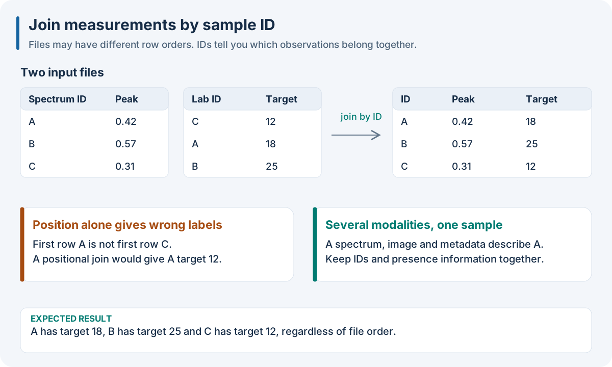
Align by ID, not row number. NIR, image and metadata rows can occur in different orders. The join restores the same A/B/C order, so each model input describes one specimen.

Explanation: The four files can contain the same observations in different orders. Joining by stable IDs restores the same observation order before encoding. Joining row 1 to row 1 would combine measurements from different samples.

Consider a record with sample_id="A", a NIR spectrum with 400 wavelengths, an image with shape (32, 32, 3), a series with shape (50, 2), and metadata [temperature, instrument]. These widths and shapes describe distinct representations; flattening and concatenating everything without a declared encoder would erase their semantics and may give a large source unintended weight.

Source	Preserve in the raw schema	Typical encoder question
NIR	Ordered wavelength coordinates, units and signal type	Scale, correct scatter or derive the signal?
Image	Height/width/channel axes, dtype and coordinates where applicable	Learn a compact tensor representation?
Series	Time axis, channels, length/offsets and time units	Fixed-shape tensor PCA or an explicit ragged policy?
Metadata	Numeric/categorical column identity and string values	Learn scaling and a category vocabulary?
Target	Name, unit, task and validity mask	Which observations can fit and score this target?

A feature axis changing from nanometres to wavenumbers is a schema change, even if its length stays the same. A change in categorical spelling can create an unseen category. Keep these decisions in the declaration and inspect the saved predictor’s accepted schema before serving predictions.

Try the alignment yourself

These marker measurements are deliberately out of order. The JSON/YAML tabs show inputs and expected output; the language tabs perform the same join. This is host array code, which you can run before loading data into nirs4all.

JSON

{
  "spectrum_ids": [
    "A",
    "B",
    "C"
  ],
  "marker_ids": [
    "C",
    "A",
    "B"
  ],
  "marker_values": [
    30,
    10,
    20
  ],
  "aligned_marker_values": [
    10,
    20,
    30
  ]
}

YAML

spectrum_ids: [A, B, C]
marker_ids: [C, A, B]
marker_values: [30, 10, 20]
aligned_marker_values: [10, 20, 30]

Python

spectrum_ids = ["A", "B", "C"]
marker_ids = ["C", "A", "B"]
marker_values = [30, 10, 20]
lookup = dict(zip(marker_ids, marker_values))
aligned = [lookup[sample] for sample in spectrum_ids]
assert aligned == [10, 20, 30]
print(aligned)

R

spectrum_ids <- c("A", "B", "C")
marker_ids <- c("C", "A", "B")
marker_values <- c(30, 10, 20)
positions <- match(spectrum_ids, marker_ids)
stopifnot(!anyNA(positions))
aligned <- marker_values[positions]
print(aligned) # 10 20 30

Octave / MATLAB

spectrum_ids = {'A', 'B', 'C'};
marker_ids = {'C', 'A', 'B'};
marker_values = [30, 10, 20];
[found, positions] = ismember(spectrum_ids, marker_ids);
assert(all(found));
aligned = marker_values(positions);
disp(aligned); % 10 20 30

WASM / JavaScript

const spectrumIds = ['A', 'B', 'C'];
const markerIds = ['C', 'A', 'B'];
const markerValues = [30, 10, 20];
const lookup = new Map(markerIds.map((id, i) => [id, markerValues[i]]));
if (spectrumIds.some(id => !lookup.has(id))) throw Error('Missing marker ID');
const aligned = spectrumIds.map(id => lookup.get(id));
console.log(aligned); // [10, 20, 30]

Expected result: marker values become [10, 20, 30] beside spectra A, B and C. Without the join, A would be assigned C’s value 30. Before a real join, also reject duplicate IDs and choose an explicit policy for missing IDs; the tiny exercise assumes unique complete IDs.

Missingness is part of the modeling problem

Situation	Example	Decision required
Missing source	Sample A has no image	Choose a profile supporting missing modalities and its fusion policy
Missing feature	One wavelength value is invalid	Choose an explicit imputation/validity policy accepted by the operator
Missing target	A reference assay was not performed	Use a supported target-mask/per-target profile
Ragged source	Series A has 45 points and B has 61	Preserve offsets/time, then choose an explicit encoder/aggregation policy
Repetition	Three spectra of the same specimen	Preserve origin/group IDs and keep the specimen within one CV side
Derived sample	A noise-augmented version of A	Preserve origin identity and restrict fitting/evaluation accordingly

Zero-filling a missing modality turns absence into a measurement. Zero-filling an unobserved target changes the scientific outcome. Even if a loader can assemble the data, the chosen training profile must accept the masks and representations. Consult Public execution matrix before combining ragged inputs, missing sources, partial targets and native export.

Read the portable JSON document

The common download in 1. Run your first complete experiment is a complete runnable example of two nested declarations: the outer nirs4all.dataset.v1 wrapper carries origin and fold identities; its dataset member is a nirs4all.multimodal-dataset value. The source contains a typed array with dtype, shape and values, ordered sample_ids, representation_id, axes, and coordinate metadata. y and partitions are also typed arrays.

Explanation: The wrapper keeps execution identities, while the dataset describes the aligned observations, source schemas, targets and partitions. A pipeline recipe remains a separate object.

The Python Core, R, WASM and Octave tabs in 1. Run your first complete experiment consume this document through their dataset APIs. Keep the complete downloaded JSON when running that tutorial; this diagram is a schema-reading aid, not a replacement file.

Build up to the four-source training example

The executable U07_multimodal.py progresses from typed sources to training, search, export and replay. Its Methods early-fusion profile fits StandardScaler on NIR, TensorPCA on image and series, a numeric scaler and one-hot vocabulary on metadata, then Ridge on weighted concatenated encodings. Fold encoders are learned on training rows. The full refit archive includes those encoders, not only Ridge coefficients.

For this specific Methods profile, use complete fixed-shape sources, one complete numeric target named y, three grouped folds and a full refit. It is not the ragged/missing-source profile. Follow Native multimodal early fusion for its parameter grid and exact limits, then Fusion tardive avec observations partielles for a separate partial-cohort workflow.

Before fitting, verify sample counts per source, target coverage, group counts, partition sizes, dtype and non-sample shape. Before replay, verify the same source names, feature identity, units and axis coordinates independently of array shape.

Dataset checklist before training

1. State what one row represents and the independent validation unit.

2. Count rows and features; keep target values outside the feature table.

3. Join sources by unique sample IDs; compare IDs after the join.

4. Preserve wavelength/time coordinates, feature names and units.

5. Keep missing sources, missing feature values and missing labels distinct.

6. Declare train/test partitions before comparing recipes.

Checkpoint: explain why image row 1 might not belong beside spectrum row 1. Continue to 5. Build a pipeline you can explain.