9. Choose transforms and models for a reason

Your goal: connect a visible measurement problem to a candidate operation, then test whether that choice helps held-out predictions. Begin with a simple baseline; complexity should answer a specific question.

A preprocessor changes what the model sees. A model changes the relation you try to learn. A smooth spectrum or a low training error is not, by itself, evidence of better future predictions.

Choose an operator by its role in the workflow: preprocessing, feature selection, splitting, filtering, augmentation, prediction, optimization or diagnosis. Then check the host/runtime, parameter types and artifact profile for that operator.

Role	Reference	Questions to answer
Spectral preprocessing	Transforms Reference	Required axis, wavelength spacing, learned state and numerical convention
Regression/classification	Built-in Models Reference	Task, target shape, scale assumptions and serialization
Native Methods catalog	Methods catalog	Exact native ID, parameters, supported binding and ABI
Splitters	Splitters Reference	Unit of independence, stratification, groups and determinism
Filters/selection	Filters Reference	Fit scope, row/feature removal and leakage policy
Augmentation	Augmentation Operators Reference	Training-only scope, origin identities and stochastic seed
Search	Generator keywords: choices, combinations and their exact outputs	Expansion or adaptive optimization, constraints and resume
Diagnostics/intervals	6. Measure whether your model answers the question	Complete predictor versus branch, calibration evidence and audit purpose

The operator catalog and node reference provide categorized discovery. They are not a guarantee that every operator can execute in every language. A Methods binding exposing a kernel does not automatically expose it through a nirs4all task facade.

Detailed parsing, numerical and orchestration references belong to their upstream projects: Formats, IO, Methods, DAG-ML and DAG-ML-Data. This guide explains how those components participate in a complete user workflow.

Understand what a method changes

An operator implements a numerical operation. A node places it in the workflow. A controller manages its data layout, fit scope and fitted state. For example, SNV() is an operator used as a preprocessing node; wrapping a noise operator in sample_augmentation gives it training-only semantics. Moving the same operator into another container can change the resulting dataset, even when its numerical formula stays the same.

The decision sequence is question → operation → orchestration → capability check → evaluation → fitted export. A list of available class names answers only the second of these questions.

Learn preprocessing by observing its effect

SNV changes values without adding rows or columns. Spectrum A has mean 2 and population standard deviation about 0.816; B has mean 5 and standard deviation about 1.633. After subtracting the mean and dividing by the spread, their normalized shapes coincide. These three-point spectra illustrate the arithmetic, not predictive performance.

SNV subtracts each spectrum’s own mean and divides by its own standard deviation. MSC instead fits a reference spectrum from training rows and estimates each row’s offset and slope against that reference. A derivative removes a constant offset but amplifies short-scale noise. Consequently, SNV, MSC and derivatives address related problems through different mechanisms. Evaluate them as alternatives before chaining all of them.

Observation in raw data	Candidate experiment	What to inspect after fitting
Additive offset or gain between repeated acquisitions	SNV, MSC, EMSC	Whether relevant concentration differences were also removed
Smooth baseline drift	Detrend, polynomial or asymmetric baseline correction	Peak integrity and residual baseline
High-frequency detector noise	Savitzky–Golay, Gaussian, wavelet denoising	Narrow peaks, boundaries, smoothing bias
Broad background conceals slopes or shoulders	Smoothed first/second derivative	Noise amplification and wavelength spacing
Dense correlated wavelengths	PLS, PCA/SVD followed by a model	Validation error versus retained dimensions
Many irrelevant channels	CARS, MCUVE, sparse/interval PLS	Selection stability across training folds
Sensor grids differ	Physical resampling and documented cropping	Grid overlap, extrapolation and coordinate units

Read Transforms Reference for the operator families, fit-state rules, parameter interpretation and a complete executable transformation example. The tracked U01_preprocessing_basics.py, U04_signal_conversion.py, U05_orthogonalization.py and U06_wavelet_denoise.py explore these decisions.

Choose model complexity by evidence

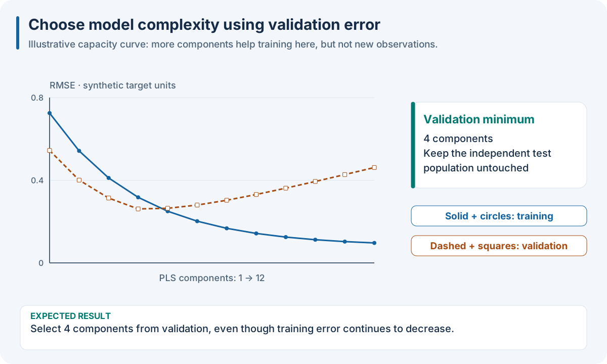
An illustrative capacity curve, computed from explicit synthetic formulas. The validation minimum is four components. No measured benchmark is represented.

PLS learns directions that relate X to y; PCA learns directions of high X variance without looking at y. Increasing components may explain more training variation while worsening generalization. A component count must also fit the rank and sample count of the smallest training fold. Search on development folds, then score the selected complete predictor on independent test data.

Family	Useful hypothesis	Main cost or failure mode
PLS/SIMPLS/IKPLS	A few latent directions capture a mostly linear calibration	Too many components fit noise; scaling conventions affect coefficients
Ridge/linear regression	Many correlated predictors have a smooth linear effect	Regularization and feature scaling need validation
Sparse/interval PLS	Only some wavelengths carry stable predictive information	Channel selection can be unstable on small folds
OPLS/OSC plus PLS	A large part of X variation is unrelated to y	Supervised filtering must stay inside training folds
Kernel PLS/SVR	Relationships are nonlinear but samples are limited	Kernel scale and regularization are sensitive; dense kernels use quadratic memory
Random forests/boosting	Thresholds and interactions matter	Extrapolation outside training ranges is weak
AOM/POP/FastAOM	Preprocessing choice should be learned with the calibration	Internal model selection adds CV and resource cost
MBPLS/early fusion	Sources contain complementary feature information	Large or highly scaled blocks can dominate
Stacking/late fusion	Source-specific predictors make complementary errors	The final model must learn from out-of-fold predictions
Neural models	Enough data justify representation learning	Dependency, device, stochasticity and fitted-artifact profile

Follow Built-in Models Reference and U04_pls_variants.py for model parameters; U07_aom_panoply.py demonstrates adaptive families. Classification needs class outputs and appropriate metrics; a regressor thresholded after selection is not automatically a calibrated classifier.

Augmentation is an assumption about future measurements

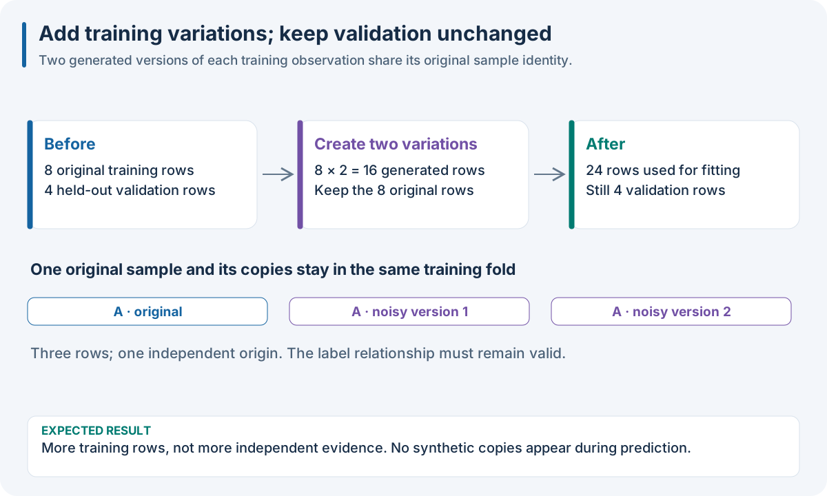
Augmentation adds training variations, not independent evidence. Eight originals plus sixteen derived rows give 24 rows used for fitting. All versions keep their original specimen relationship. The four held-out validation observations receive no synthetic siblings.

Specify a plausible nuisance mechanism: noise level, instrument offset, wavelength drift, missing detector band or optical path length. Choose its magnitude in the units used by the input. A perturbation that destroys the target relationship creates mislabeled training data. Augment training rows after their independent origins have been separated from validation; compare against an unaugmented baseline using identical folds. See Augmentation Operators Reference and U03_sample_augmentation.py.

Estimate a search before running it

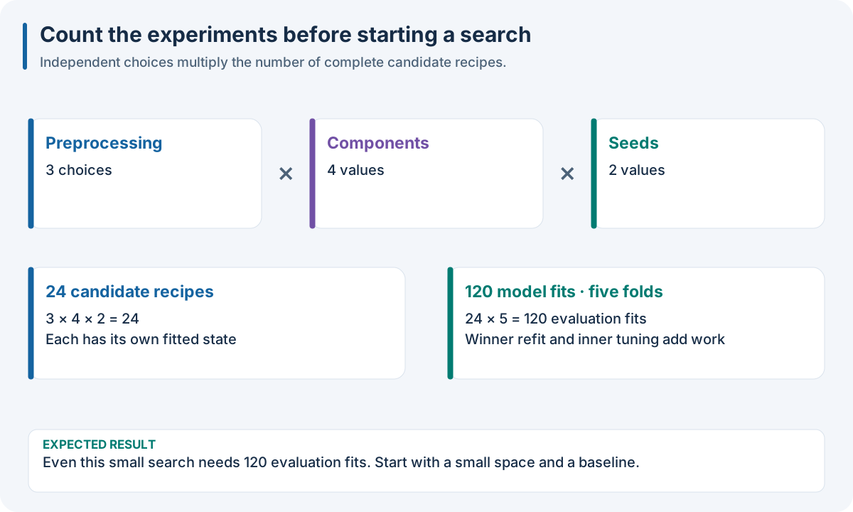
Cartesian search arithmetic: 3 × 4 × 2 = 24 recipes. Five evaluation folds multiply this to 120 model fits; nested CV and adaptive banks add further fits.

Alternatives generate separate candidate recipes. Branches keep multiple paths within a recipe. This distinction determines both the computational budget and what gets exported. Start with a small reproducible grid and a simple baseline. Introduce adaptive optimization, structural search and ensembles only when the prior experiment identifies a reason to do so. The 5. Build a pipeline you can explain chapter and Generators: turn an experiment plan into concrete recipes explain composition, constraints, seeds and why a search definition is not fitted state.

These figures use explicit teaching values to illustrate numerical changes, observation counts and search arithmetic. The capacity curve is illustrative, not a measured benchmark.

Open a worked node before choosing its parameters

I need to…	Open…	Observe…
Remove spectrum-wise offset/gain	preprocessing	Raw versus corrected spectra
Scale a target and return original units	target processing	Model-scale y versus final predictions
Compare model sizes	generators	Expanded list of candidate recipes
Keep complementary sources	branch and merge	Each source’s columns and the joined matrix
Combine distinct predictors	prediction merge	OOF prediction columns used by the final model
Simulate plausible acquisition noise	sample augmentation	Derived rows and unchanged origin relationships
Select or flag suspicious observations	tag and exclude	Which training observations remain
Correct a base model’s remaining error	residual model	Base estimate plus learned correction

Checkpoint: explain which nuisance your operation addresses, what values or dimensions it changes, and how you will compare it with the baseline. Continue to 10. Run the same recipe in your language.