6. Measure whether your model answers the question

Your goal: choose a validation split, calculate its error, and distinguish the score used to select a recipe from the score used to assess the final predictor.

Ask first: what will the next unknown observation be? Another scan of a known specimen, a new specimen, a new batch or a new instrument? The split should imitate that situation. If specimens have repeated scans, separate specimens rather than random rows.

Keep partitions distinct

Evidence	Use	Avoid
Training predictions	Diagnose fitted behavior	Treating them as held-out accuracy
Validation/OOF predictions	Candidate selection and stacking	Fitting preprocessing on validation rows
Test predictions	Final external evaluation	Selecting repeated candidates on test scores
Refit state	Deploy the selected recipe	Reusing a fold model as the complete predictor
Calibration predictions	Fit a conformal calibrator	Training the point model on the calibration labels
New-data prediction	Apply fixed learned state	Reconstructing or refitting hidden encoders

Specify the objective and direction together: minimize error/loss, maximize the chosen score where appropriate. Report per-target results and validity masks for partial/multiple targets. Aggregating groups, repetitions or folds requires a declared aggregation policy and must preserve the original sample/unit identities.

Add intervals only after the point predictor is fixed

Suppose a held-out calibration set gives a supported 90% residual allowance of 2 concentration units. A new point prediction of 10 receives interval [8, 12]. The allowance is learned from calibration errors using the conformal method’s finite-sample rule; it is not the training RMSE copied into a band. Assess actual coverage on another labeled cohort.

Conformal intervals

Split-conformal calibration uses a fitted point predictor and an explicitly separate observed calibration cohort. Export includes the calibrator’s method, exchangeability unit, supported coverage levels and cohort provenance. predict_calibrated applies it to future point predictions. conformal_metrics reports observed coverage and interval widths where truth is available.

Calibration support is profile-specific. A browser consuming a CPU archive already calibrated is different from calibrating a previously uncalibrated CPU archive in the browser. Consult the current transport matrix in 8. Save a predictor and use it on new observations. Do not infer one from the other.

Robustness and visual reports

A frozen robustness audit evaluates declared slices or perturbation scenarios against a fixed clean predictor. It does not replace the model or claim robustness to every distribution change. Retain the scenario definition, seed where applicable, reference cohort and metrics.

Use a chart when it helps explain a result, and accompany it with a visible conclusion and the values needed to check it. Identify units, partitions, target names and missing values. Color alone must not distinguish models or uncertainty. Exported figures need their own text alternative or adjacent data table.

For examples, see Understanding Scores, Evaluation, and Refit, Metrics Reference, Native tuning and conformal calibration and Analyzer Charts Reference. Multimodal SHAP for the complete refit predictor remains a separate deferred work item; explanations of one feature branch are not complete-model explanations.

Select a splitter for the prediction question

Intended prediction	Starting splitter	Why	Check
New independent observations from the same population	KFold or ShuffleSplit	Random held-out evaluation	Independence and sufficient training size
New specimens with repeated scans	GroupKFold	All scans of a specimen stay together	Group IDs really identify specimens
Imbalanced categorical outcome	StratifiedKFold	Keeps classes represented	Every fold has enough class observations
Imbalanced outcome with specimen groups	StratifiedGroupKFold	Combines class balance and group separation	Balance may be constrained by groups
Future measurements	TimeSeriesSplit or explicit chronological holdout	Respects the direction of time	No preprocessing or labels from the future
New laboratory/instrument/batch	Explicit held-out groups	Tests the acquisition shift of interest	Enough independent groups for the conclusion

Splitter availability and grouping syntax depend on the execution profile. The SDK U01_cv_strategies.py and U02_group_splitting.py provide worked examples. The latter explicitly uses the legacy profile for its automatic repetition-grouping demonstrations; do not transplant those settings to native Core without checking its profile.

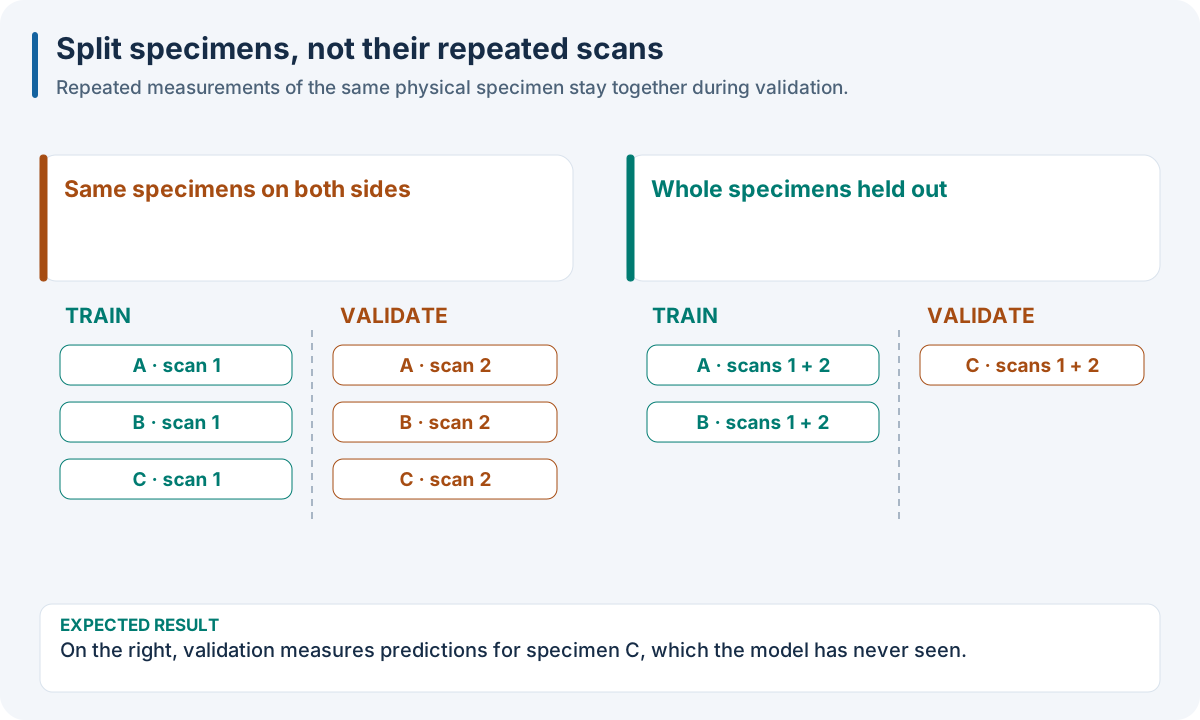
Repeated scans of the same specimen stay together in a fold so validation tests new specimens. — **Match validation to deployment.** All scans of a held-out specimen remain outside training. The scaler and model learn only from training specimens; held-out scans use the fixed learned state.

Explanation: Every scan of specimen B belongs to the validation side; specimens A and C belong to training. The figure illustrates one fold, not a claim that three specimens are enough for a scientific study. This protocol asks about a new specimen rather than another scan of a known specimen.

Work through pooled error by hand

For regression, with residual r = prediction - truth, RMSE is the square root of the mean squared residual. Its unit is the target unit. MAE is the mean absolute residual; it weights large deviations less strongly. R² compares the squared residuals with target variability and can be negative. A favorable R² alone does not demonstrate sufficiently small error for your application.

Here is a deliberately small illustrative calculation, not an experiment result:

Fold	Held-out residuals	Count	Sum of squared residuals	Fold RMSE
0	1, 1	2	2	1
1	3, 3	2	18	3
Pooled	1, 1, 3, 3	4	20	√5 ≈ 2.236

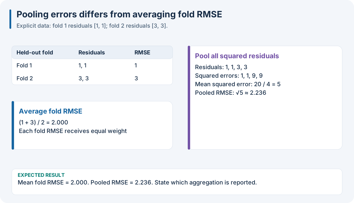
Fold RMSEs of 1 and 3 average to 2, while pooling their four residuals gives RMSECV of approximately 2.236. — Illustrative RMSE aggregation, in arbitrary target units. The two folds have the same size; their pooled RMSE still differs from the mean fold RMSE. The table above supplies the full residuals and values. These are teaching values, not measured nirs4all performance.

The mean fold RMSE is (1 + 3) / 2 = 2. The pooled RMSE is sqrt((2 + 18) / 4) ≈ 2.236. They answer different aggregation questions; unequal fold sizes introduce an additional weighting difference.

Explanation: Pooling residuals before taking the square root produces approximately 2.236; averaging fold RMSEs produces 2. The table above contains all values needed to reproduce the diagram.

KFold gives each observation one validation prediction per complete CV pass. ShuffleSplit and repeated CV can produce several held-out predictions for one observation or leave some observations unvalidated. Keep fold membership and prediction multiplicity visible; choose the supported aggregation policy rather than assuming all CV evidence is one row per observation.

Calculate the error in your language

The inputs below give residuals 1, 1, 3 and 3. JSON/YAML show the same values and expected answer. The executable tabs use the definition directly, so the error calculation does not depend on a particular model API.

JSON

{
  "truth": [
    10,
    12,
    14,
    16
  ],
  "prediction": [
    11,
    13,
    17,
    19
  ],
  "residual": [
    1,
    1,
    3,
    3
  ],
  "rmse": 2.23606797749979,
  "mae": 2
}

YAML

truth: [10, 12, 14, 16]
prediction: [11, 13, 17, 19]
residual: [1, 1, 3, 3]
rmse: 2.23606797749979
mae: 2.0

Python

import numpy as np
truth = np.array([10, 12, 14, 16])
prediction = np.array([11, 13, 17, 19])
residual = prediction - truth
print("RMSE:", np.sqrt(np.mean(residual ** 2)))
print("MAE:", np.mean(np.abs(residual)))

R

truth <- c(10, 12, 14, 16)
prediction <- c(11, 13, 17, 19)
residual <- prediction - truth
print(sqrt(mean(residual^2))) # RMSE = 2.236068
print(mean(abs(residual)))   # MAE = 2

Octave / MATLAB

truth = [10, 12, 14, 16];
prediction = [11, 13, 17, 19];
residual = prediction - truth;
disp(sqrt(mean(residual.^2))); % RMSE = 2.236068
disp(mean(abs(residual)));     % MAE = 2

WASM / JavaScript

const truth = [10, 12, 14, 16];
const prediction = [11, 13, 17, 19];
const residual = prediction.map((p, i) => p - truth[i]);
const rmse = Math.sqrt(residual.reduce((s, r) => s + r*r, 0) / residual.length);
const mae = residual.reduce((s, r) => s + Math.abs(r), 0) / residual.length;
console.log({rmse, mae}); // 2.23606797749979, 2

Expected result: RMSE ≈ 2.236 and MAE = 2, in the target’s unit. These values are illustrative and were chosen to make the pooled calculation visible.

Separate selection from the final score

cv_best_score identifies CV selection evidence in the SDK result. final_score refers to the refit predictor’s test evidence where that cohort exists. best_score is a convenience accessor; inspect its associated entry and metric rather than treating the name as a complete definition of the protocol. The detailed Understanding Scores, Evaluation, and Refit distinguishes pooled CV score, mean fold validation score, fold-ensemble test score and refit test score.

JSON