Learn to build, understand and reuse pipelines

Start with one complete experiment. End with several sources, branches, a model search and a saved predictor. This course is for people who know their measurements and want to understand every step between a raw observation and a prediction. Follow it from Python, R, Octave or a browser.

Our question is “Can these measurements predict the concentration of a sample?” A pipeline is the recipe: prepare inputs, train a model, check predictions on observations it has not seen, and save the selected model. Images, time series and laboratory metadata can join the spectrum later.

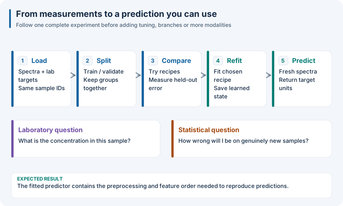
The complete journey. Validation answers which recipe to keep. The final fit creates the predictor you reuse. Future observations use its learned transformations and coefficients.

Choose your starting point

1 · Run a first experiment

Install your tools, fit a small model and save a result you can reload.

1. Run your first complete experiment

2 · Understand the data

Read rows, columns, IDs, groups and multiple sources. Align them correctly.

4. Describe your measurements and align your sources

3 · Explore every pipeline node

A clickable catalogue: purpose, input/output, example and illustration.

Choose a pipeline node by what you want to do

4 · Build and compare recipes

Generate candidates, branch the data, merge features and build stacking.

5. Build a pipeline you can explain

5 · Read the evidence

Know which score answers your question and what your figures should reveal.

6. Measure whether your model answers the question

6 · Predict in your language

Use a shared recipe in Python, R, Octave and WASM; export and reload.

10. Run the same recipe in your language

Follow the course in order

Chapter	You will learn to…	Check before continuing
0. Choose the tools for your language	Choose your language’s installed product	Identify the package you actually call
1. Run your first complete experiment	Train and save a predictor	Find two candidates and a saved model
2. Understand what the pipeline learns	Explain learning, validation and refit	Distinguish settings from learned coefficients
3. Choose the operation you need	Choose run, generate, predict or retrain	State what you have and what you need
4. Describe your measurements and align your sources	Describe one or several measurement sources	Match IDs and explain one row
5. Build a pipeline you can explain	Combine nodes and compare alternatives	Draw the data reaching each model
6. Measure whether your model answers the question	Choose folds and interpret scores	Keep a specimen on one side of a split
7. Read the result and keep a useful experiment record	Make a scientific report	Identify the winner and its evaluation data
8. Save a predictor and use it on new observations	Reload the complete predictor	Predict without fitting again
9. Choose transforms and models for a reason	Choose preprocessing and models	Explain the expected signal change
10. Run the same recipe in your language	Run the shared example in your language	Compare values and row identities
11. Progress from a baseline to an advanced workflow	Assemble an advanced workflow	Complete branching and source-fusion exercises
12. Add an operation or contribute an example	Add an operation when needed	Locate numerical code and its tests
13. Find a node, parameter, example or solution	Look up exact keywords and parameters	Reach the relevant example directly

How to read the examples

Each code box groups all applicable languages in synchronized tabs: JSON/YAML recipes and Python, R, Octave/MATLAB or WASM/JavaScript execution where supported. Your selection follows you between chapters. Runtime limitations and executable alternatives are explained beside the examples; installation tabs contain only actual language tools.

The shared recipe uses native method IDs. Advanced Python recipes use sklearn-compatible objects. They are two supported ways to work with different operator coverage; 0. Choose the tools for your language explains the choice.

Figures explain changes to data and expected results. Synthetic examples make arithmetic inspectable; their curves and scores are teaching examples, not claims about your instrument.