11. Progress from a baseline to an advanced workflow

Your goal: complete seven practical stages, each adding one mechanism you can explain. You may stop at the simplest stage that answers your scientific question. The final exercise combines source-specific preprocessing, fusion and correction, then tests saved-model replay.

Keep an experiment notebook with inputs, recipe, split, figure and conclusion. When an example is Python-only, use its native counterpart in 10. Run the same recipe in your language for the shared operations; the tabs mark actual availability.

Recipe	Executable guide	What to retain
First regression and candidate selection	1. Run your first complete experiment and Quickstart	Dataset, candidates, OOF, selected refit and export
Compare preprocessing and models	Preprocessing Examples and Model Examples	Comparable validation protocol and metric direction
Cross-validation and grouped observations	Cross-Validation Examples and Sample Repetition & Aggregation	Group/repetition/origin IDs and fold memberships
NIR + image + series + metadata	Native multimodal early fusion	Encoder state, schema, fusion model and no-FIT replay
Partial cohorts and late fusion	Fusion tardive avec observations partielles	Source/target masks and held-out meta-model inputs
Native R/Octave host workflow	Octave models in a Python multimodal workflow	Host artifact manifests, native scores and fresh-process replay
Optimize, resume, refit and export	Native PLS HPO within each outer fold and Search source subsets, preprocessing chains and Ridge versus PLS	Search contract, parent/checkpoint identity and refit state
Conformal intervals	Native tuning and conformal calibration	Calibration cohort, calibrator and observed coverage
Reuse/deploy a selected model	Deployment Examples	Frozen input schema and portable/host-specific artifact profile
Native pipeline, SDK workspace and browser/CPU transport	Move a native model or a complete experiment	Profile/version, masks, native state, SDK snapshot and closeable sessions

The examples index connects runnable examples with guides. Synthetic datasets illustrate behavior and support deterministic qualification; they do not substitute for evidence on a real acquisition or instrument. Label that distinction in reports and charts.

A successful producer run is only half of an interlanguage tutorial. Verify the actual exported bytes and repeat prediction in the target language with fitting disabled and no access to the training workspace.

Work through the stages in order

Complex pipelines become manageable when each added mechanism has a purpose and a check. Keep the same IDs and evaluation protocol until the lesson explicitly changes them. The following stages form a practical learning path, not a claim that a single API accepts every configuration in every language.

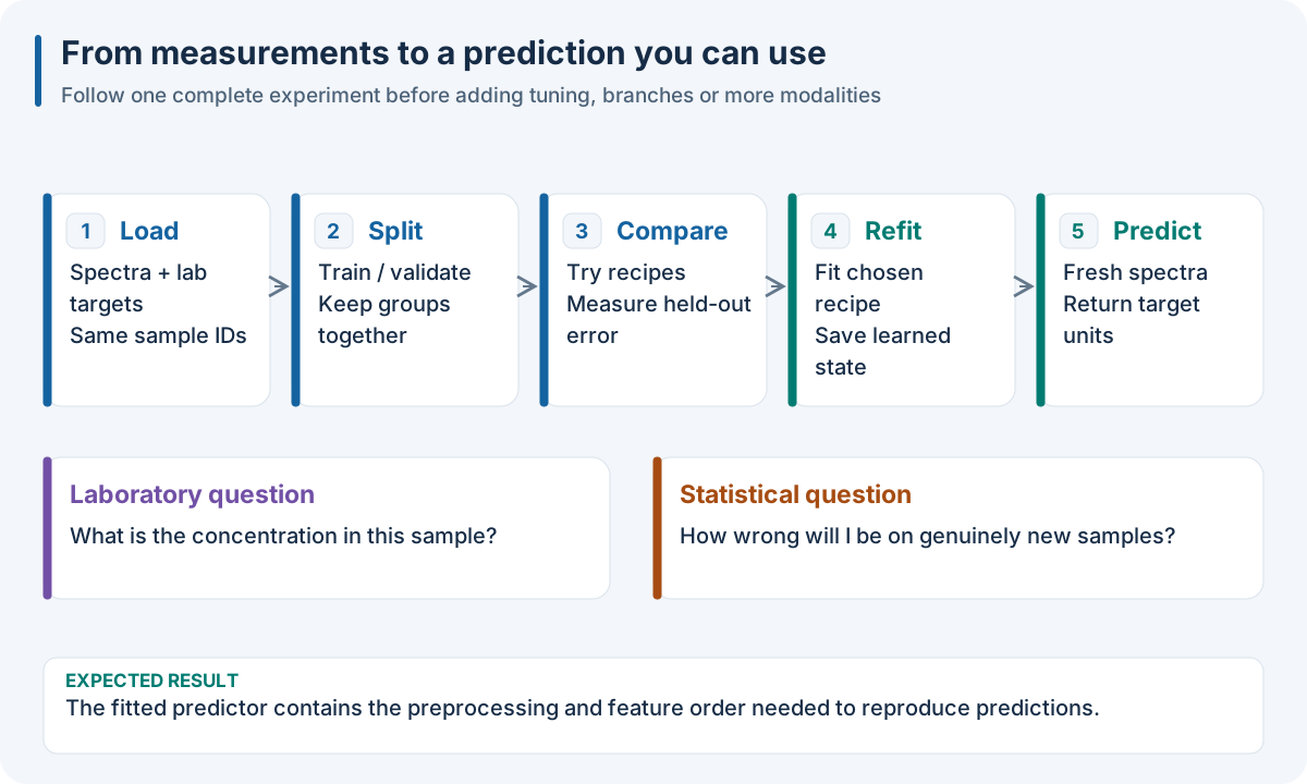
The learning sequence goes from a baseline through validation and selection to a reusable predictor. — **Build one understanding at a time.** First explain the input/target and validation. Then add transforms, groups, branches and sources. Finish by reloading the complete learned predictor.

Explanation: learn how a single model is evaluated, then how transforms, identity, branches and multiple modalities change its inputs. Optimize and calibrate only after that protocol is understood. Finish by replaying the selected fitted state in the intended deployment language.

Stage 1 — Read the data contract and fit a baseline

Run 1. Run your first complete experiment in your language, then the finite Ridge recipe in 10. Run the same recipe in your language. State what one row represents, the target’s physical unit and whether observations are independent. Identify X, y, sample IDs, source IDs, partitions and target names before fitting. The downloadable twelve-row dataset is synthetic; its score demonstrates software behavior.

Checkpoint: explain why a validation prediction uses a model fitted without that row, why full refit follows selection and why the deployment predictor has no need for labels. Inspect the selected candidate and exported artifact, then reload it. Compare sample_ids and target_names, not just the numeric array.

Stage 2 — Compare preprocessing without changing the question

Follow Preprocessing Examples and Preprocessing Overview. Start with a fixed model and fixed folds. Add SNV to suppress sample-wise scatter effects, then try a Savitzky–Golay smoother or derivative with explicit window/order parameters. Plot raw and transformed spectra against the same wavelength coordinates. A derivative changes the signal and its interpretation; a visually smooth spectrum alone does not establish predictive improvement.

Checkpoint: distinguish a row-wise transform (SNV) from a learned feature-wise transform (standardization). Explain which values are estimated on the training fold, which parameters are predetermined and which choices are selected by held-out scores. Compare RMSE using the same folds and target unit.

The executable Python examples are examples/user/03_preprocessing/U01_preprocessing_basics.py, U02_feature_augmentation.py and U03_sample_augmentation.py in the same folder. Feature augmentation creates additional feature views; sample augmentation creates training observations whose origin IDs must remain known. An augmented sibling of a validation sample must not enter the training fold.

Stage 3 — Preserve groups and repetitions

Follow Cross-Validation Examples and Sample Repetition & Aggregation. If several spectra come from one physical specimen, a random row split can place the same specimen in training and validation. The score then answers a different, easier question. Choose the independent unit that matches deployment and split that unit.

For the portable dense fixture, this Python exercise declares six two-row groups and three fold assignments. It illustrates contract construction; replace the artificial groups with acquisition identities in real work:

JSON

{
  "dataset.groups": {
    "dtype": "<U3",
    "shape": [
      12
    ],
    "values": [
      "g0",
      "g0",
      "g1",
      "g1",
      "g2",
      "g2",
      "g3",
      "g3",
      "g4",
      "g4",
      "g5",
      "g5"
    ]
  },
  "fold_ids": [
    "f0",
    "f0",
    "f1",
    "f1",
    "f2",
    "f2",
    "f0",
    "f0",
    "f1",
    "f1",
    "f2",
    "f2"
  ]
}

YAML

dataset.groups:
  dtype: <U3
  shape:
  - 12
  values:
  - g0
  - g0
  - g1
  - g1
  - g2
  - g2
  - g3
  - g3
  - g4
  - g4
  - g5
  - g5
fold_ids:
- f0
- f0
- f1
- f1
- f2
- f2
- f0
- f0
- f1
- f1
- f2
- f2

Python

import json
from pathlib import Path
from nirs4all_core import run_pipeline

record = json.loads(Path("dataset.json").read_text())
recipe = json.loads(Path("ridge.recipe.json").read_text())
count = len(record["origin_ids"])
record["dataset"]["groups"] = {
    "dtype": "<U3", "shape": [count],
    "values": [f"g{i // 2}" for i in range(count)],
}
record["fold_ids"] = [f"f{(i // 2) % 3}" for i in range(count)]
model = run_pipeline(record, recipe)
ids = record["origin_ids"]
groups = dict(zip(ids, record["dataset"]["groups"]["values"]))
for fold in model.outcome["effective_plan"]["fold_set"]["folds"]:
    training = {groups[s] for s in fold["train_sample_ids"]}
    validation = {groups[s] for s in fold["validation_sample_ids"]}
    assert training.isdisjoint(validation)

R

library(nirs4all)
record <- jsonlite::fromJSON("dataset.json", simplifyVector = FALSE)
recipe <- jsonlite::fromJSON("ridge.recipe.json", simplifyVector = FALSE)
record$dataset$groups <- list(dtype = "<U3", shape = list(12L),
  values = as.list(paste0("g", rep(0:5, each = 2))))
record$fold_ids <- as.list(paste0("f", rep(c(0, 1, 2, 0, 1, 2), each = 2)))
model <- nirs4all_run_pipeline(record, recipe)
print(model$outcome$effective_plan$fold_set$folds)

Octave / MATLAB

record = fileread('dataset.json');
recipe = fileread('ridge.recipe.json');
% Replace only these fields, preserving exact array declarations elsewhere.
groups = ['{"dtype":"<U3","shape":[12],"values":' ...
  '["g0","g0","g1","g1","g2","g2","g3","g3","g4","g4","g5","g5"]}'];
folds = '["f0","f0","f1","f1","f2","f2","f0","f0","f1","f1","f2","f2"]';
record = regexprep(record, '"groups"\s*:\s*null', ['"groups":' groups], 'once');
record = regexprep(record, '"fold_ids"\s*:\s*\[[^\]]*\]', ['"fold_ids":' folds], 'once');
model = nirs4all.runPipeline(record, recipe);
disp(model.outcome.effective_plan.fold_set.folds);

WASM / JavaScript

import {runBrowserPipeline} from 'nirs4all';
const record = await (await fetch('./dataset.json')).json();
const pipeline = await (await fetch('./ridge.recipe.json')).json();
record.dataset.groups = {dtype: '<U3', shape: [12],
  values: Array.from({length: 12}, (_, i) => `g${Math.floor(i/2)}`)};
record.fold_ids = Array.from({length: 12}, (_, i) => `f${Math.floor(i/2)%3}`);
const model = await runBrowserPipeline(record, {pipeline});
console.log(model.outcome.effective_plan.fold_set.folds);

The JSON/YAML tabs show the two changed fields, not a full dataset document: dataset.groups names the nested field and fold_ids remains at the outer level. Apply these changes to the downloaded twelve-row record. The Octave tab edits only the two declared fields in the exact JSON text so singleton shape arrays elsewhere remain arrays.

Expected result: six groups of two observations, divided into three folds. Both rows of each group have the same fold ID. The Python assertions inspect the effective plan and confirm no group appears on both sides.

Checkpoint: remove fold_ids and check that grouped native execution refuses an implicit unsafe split. Describe whether prediction is scored per observation or after specimen aggregation. Keep group, repetition and origin identity separate; each describes a different relationship.

Stage 4 — Branch, merge and stack

Read Pipeline Branching, Branch Merging and Meta-Model Stacking User Guide. A branch creates parallel paths or separates observations by a declared condition. Merging features concatenates compatible feature views; merging predictions constructs model outputs for another estimator. Neither operation should quietly reorder samples.

For stacking, use the worked example examples/user/04_models/U03_stacking_ensembles.py. Read the feature/prediction merge before copying its pipeline. Each meta-training row must contain a base-model prediction made without fitting on that row. Predictions from full-data fitted base models are useful for deployment, but would leak information if used to train the meta-model on those same observations.

Checkpoint: draw the sources of each meta-feature and locate its OOF prediction. Explain what gets refitted when the winner is selected: base models, meta-model and any fitted preprocessing. Confirm the merge carries IDs rather than relying on incidental row positions.

Stage 5 — Add typed modalities and missing sources

Run Native multimodal early fusion before Fusion tardive avec observations partielles. The first introduces NIR, image, time-series and metadata encoders with explicit axes and fitted state. The second introduces partial cohorts and late fusion. Read examples/user/02_data_handling/U08_multimodal_targets.py, U09_multimodal_missing_sources.py and U10_multimodal_late_tuning.py alongside their guides.

Explanation: each modality retains its own representation and encoder. Fusion joins encoder outputs or OOF model outputs by sample identity, using explicit source presence and target observation masks. Missing imagery is not a valid all-zero image, and an unobserved target is not a target value of zero.

Checkpoint: inspect raw shapes, encoded dimensions, missing-source behavior and target masks. Explain whether you are using early fusion of features or late fusion of predictions, and how a sample missing one modality is treated. For Octave native workflows, continue with Octave models in a Python multimodal workflow; keep its host artifact profile distinct from the all-Methods example.

Stage 6 — Tune structure, then calibrate

Use Native PLS HPO within each outer fold for fold-safe PLS tuning and Search source subsets, preprocessing chains and Ridge versus PLS for changes in sources, encoders, preprocessing chains and fusion topology. The corresponding examples include U17_structural_hpo_ridge_pls.py, U18_structural_hpo_preprocessing_chains.py, U19_structural_hpo_source_subsets.py, U20_structural_hpo_typed_modalities.py and U21_structural_hpo_early_late.py under examples/user/04_models/.

Changing topology changes both the hypothesis being tested and its fitted state. Record the search space, trial budget, metric direction and seed. A resume checkpoint carries the original study identity; editing the search and calling it a resume compromises the comparison. Nested evaluation may be needed to estimate the performance of the whole selection procedure; winning CV scores alone are optimistically selected estimates.

Then follow Native tuning and conformal calibration on disjoint calibration/test cohorts. Measure coverage and interval width on held-out data, with target units and cohort provenance in the figure caption.

Checkpoint: distinguish the fitted model, the optimizer checkpoint and the calibrator. Identify which artifact supports PREDICT, which supports search resumption and which adds uncertainty output without refitting the predictor.

Stage 7 — Assemble an advanced workflow and qualify its consumer

Run the complete D08 exercise after the code boxes in 5. Build a pipeline you can explain. It performs three separate checkpoints: 62-column feature fusion, two-column prediction stacking, and 34-column two-source residual learning. Read the expected shapes on each page before running it. Record the measured validation/test scores; do not assume complexity improves them.

Your own final workflow should declare typed sources, explicit identity-safe folds, fold-fitted preprocessing/encoders, a bounded candidate search, a fusion design, selection/full refit and a separate calibration/test cohort when intervals are needed. Draw its graph before executing it. Label each node’s accepted input, output shape and fitted-state owner. Use the executable structural examples above as the starting point for the topology that matches your data.

Checkpoint: export, close the producer, start the target-language consumer and predict target-free inputs. Follow 8. Save a predictor and use it on new observations and Move a native model or a complete experiment. Change one source unit or feature order deliberately and verify rejection. Compare values within a declared tolerance and IDs exactly. A complex training run is complete only when its selected model can be replayed with the same scientific meaning.

Keep a small experiment notebook

For every stage, retain the following record with the output rather than relying on recollection:

Field	What to write
Scientific question	Target, unit, independent unit and intended new cohort
Data	Source schemas, masks, IDs, provenance and exclusions
Evaluation	Folds/partitions, aggregation, metrics and selection rule
Pipeline	Ordered nodes, parameters, branch/merge semantics and runtime
Search	Candidates/budget, seed, study/checkpoint identity
Result	OOF scores, selected candidate, refit state and test result
Deployment	Export type, consumer cohort, replay comparison and refusals

This record also supplies the captions and provenance for your charts. It makes an impressive graph inspectable: a reader can follow where each input went, what each fitted node learned and which unseen observations justified the reported result.

Explain the final experiment without mentioning APIs

Describe: “I align spectrum and marker rows by specimen ID; normalize spectra and scale markers within training folds; join their prepared features; compare candidate model settings on held-out specimens; refit the winner; save all learned transformations; and apply the saved predictor to raw new measurements.”

Then draw your actual graph and add each node’s name, input shape and expected output. If that description and graph agree with the executed recipe, you are ready to explain the model to a collaborator.