2. Understand what the pipeline learns

You will learn: how a spectrum becomes a prediction; why validation precedes the final fit; and what to save to repeat the prediction.

Imagine 60 specimens. Each has a 12-value spectrum and a measured concentration. The spectra form X, a 60 × 12 table. Concentrations form y, a 60-value vector. We want a rule that predicts concentration from a future specimen’s spectrum.

Six words you need first

Word	Meaning	Example
Observation	One recorded measurement	A spectrum from specimen A
Feature	One model input value	Absorbance at 1,450 nm
Target	The outcome to predict	Protein concentration, in percent
Transformation	A change to the inputs	Remove a baseline or standardize a column
Model	A learned relation between inputs and target	PLS with two components
Pipeline	The ordered recipe containing these operations	Standardize → PLS

A node is a configured step. An operator is its computation, such as SNV or Ridge. A controller tells nirs4all how to fit, apply and save it. Choose the node and settings; the controller handles execution.

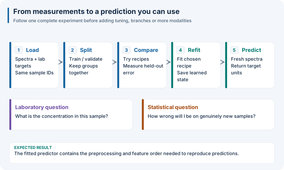
From measurements to a reusable model. Validation uses learned quantities from training rows. The full final fit follows the comparison.

Follow a single training fold

Divide 60 specimens into three groups of 20. In the first fold, train on 40 and validate on 20:

1. Estimate each feature’s mean and spread using the 40 training rows.

2. Standardize those rows using the estimated values.

3. Fit regression using their standardized features and concentrations.

4. Apply the same means, spreads and model to the 20 held-out spectra.

5. Compare those predictions with the 20 measured concentrations.

Repeat with a different held-out group. Every specimen then has a prediction from a model that did not train on it: an out-of-fold prediction, abbreviated OOF. Cross-validation, or CV, is this repeated fit-and-check process.

Calculate one transformation

One wavelength has training values 2, 4 and 6. Its mean is 4; its population standard deviation is √(8/3), about 1.633. Standardized values are approximately −1.225, 0 and 1.225. A held-out value 8 becomes (8 − 4) / 1.633 ≈ 2.449.

That held-out value does not change the training mean. Estimating the mean from all four values before validation would let evaluation information enter training: data leakage, which can make a score too optimistic.

SNV instead uses mean and spread within one spectrum. StandardScaler uses them across training spectra. Both change values, but only the latter learns across rows. See the transform node.

Select, refit, predict

Compare Ridge with alpha=0.1 and alpha=1.0. Each is a candidate, separately fitted on the same folds. Lower validation RMSE wins. The comparison does not average their coefficients.

Then fit the winning recipe on all permitted training observations. This is refit. Its learned means, scales and coefficients form the final predictor. An external test set, if declared, stays outside that fit.

For future observations, apply that saved predictor: prediction. It needs new X, no new y, and does not estimate new means from the prediction batch.

Operation	What it uses	What it produces
Fit a fold	Fold training X and y	Temporary scaler and model
Validate	Held-out X; held-out y for scoring	Candidate comparison evidence
Select	Candidate validation scores	Winning settings
Refit	All permitted training X and y	Final learned predictor
Predict	New X and saved predictor	Target estimates
Retrain	A new labeled dataset	A new predictor and experiment

Recipe, model and workspace

A recipe says “standardize, then Ridge with alpha 1.” Learned state contains the actual training means, scales, intercept and coefficients. Copying JSON reconstructs settings, not learned values. Export the fitted predictor to reuse those values.

A workspace stores experiments, scores, predictions and models together. A model export contains the predictor needed for future inputs. A session keeps runtime resources open; export saves their scientific state for later use.

Understand each source of complexity

Mechanism	What changes	Picture it as
Generator	More candidate recipes	Try SNV or MSC
Feature augmentation	More representations of the same rows	Original spectrum beside its derivative
Sample augmentation	More derived training rows	Original spectrum and a noisy copy
Branch	Several paths inside one recipe	Normalize on one path, smooth on another
Early fusion	Combine feature blocks before the model	31 spectral values + 3 markers → 34 columns
Stacking	Combine base-model predictions with a final model	Two predictions → two model inputs
Multimodal dataset	Different measurements for shared samples	Spectrum + image + metadata for specimen A

Related scans and augmented copies share an origin. Keep all observations of the same independent specimen together in a split, so validation asks about a new specimen. 6. Measure whether your model answers the question explains how.

Checkpoint: explain what is estimated in a fold and during refit, and why prediction needs the saved scaler as well as the model. Continue to 3. Choose the operation you need.