Preprocessing: change what the model sees

Use preprocessing when a measurement effect hides the information of interest: scatter, background, noise, an incompatible wavelength grid or redundant features. It transforms the feature matrix X; it leaves targets y and physical sample identity intact.

A spectrum is one row and a wavelength is one column. SNV subtracts each spectrum’s own mean and divides by its standard deviation. Spectra [1, 2, 3] and [3, 5, 7] have the same shape with different offset and gain. With the default population standard deviation (ddof=0), both become approximately [-1.225, 0, 1.225]. The matrix stays 2 rows × 3 columns.

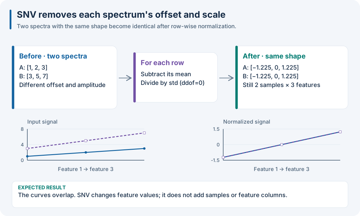
SNV removes the gain/offset distinction in this educational example. Values are rounded to three decimals.

Worked recipe

This recipe applies SNV only, exactly the operation illustrated above. Use the two short spectra for the arithmetic check, or the downloadable observations in 1. Run your first complete experiment for the complete calibration run below.

JSON

{
  "pipeline": [
    {
      "class": "nirs4all.operators.transforms.StandardNormalVariate"
    }
  ]
}

YAML

pipeline:
- class: nirs4all.operators.transforms.StandardNormalVariate

Python

from nirs4all.operators.transforms import SNV

pipeline = [SNV()]

The JSON/YAML tabs define SDK recipes; the Python tab builds the same recipe with objects. These examples use Python SDK operators. The R, Octave and browser/WASM finite pipeline facade uses native method IDs, not Python import paths. Use 10. Run the same recipe in your language for its actual binding calls and 0. Choose the tools for your language to choose the runtime.

Choices and controls

Problem	Starting operators	What to inspect
Additive/multiplicative scatter	SNV, RNV, MSC, EMSC	Relative shape after gain/offset correction
Noisy neighboring wavelengths	SavitzkyGolay(deriv=0), Gaussian, WaveletDenoise	Noise reduction and preservation of narrow peaks
Broad background	Detrend, ASLSBaseline, AirPLS, ArPLS, SNIP, RollingBall	Background subtraction and weak-band survival
Overlapping bands	FirstDerivative, SecondDerivative, NorrisWilliams, SavitzkyGolay	Slopes/curvature, noise amplification and boundary effects
Reflectance to absorbance	ToAbsorbance, ReflectanceToAbsorbance, SignalTypeConverter	Fractional reflectance 0.1 becomes absorbance 1
Too many channels	FlexiblePCA, FlexibleSVD, CARS, MCUVE	Component count or selected wavelengths
Different grids	Resampler, ResampleTransformer, CropTransformer	Coordinate units, overlap and new feature count

Form/parameter	Meaning
Direct class with params	Construct one transform in a serialized recipe
preprocessing with a transform/list	Explicitly group feature processing
Python transformer object	The same operation for interactive use
force_layout	Request 2D/3D layout for an operator that needs it
SNV axis=1	Normalize each spectrum independently
SNV with_mean, with_std, ddof, copy	Control centering, scaling, variance convention and copying
SG window_length, polyorder, deriv, delta	Window, polynomial degree, derivative order and channel spacing

Expected result of this recipe: SNV preserves sample and channel counts. The figure’s two rows both become approximately [-1.225, 0, 1.225]. Smoothing/derivatives are separate optional operations listed above: an SG derivative changes the signal interpretation and units. Its odd window must be greater than its polynomial order and fit within the available channels.

Try it: normalize the two short spectra above. Then compare SNV and MSC on offset/gain-distorted spectra: which operation needs a reference from training data?

Common mistake: normalizing away absolute amplitude when it contains the useful concentration signal. Compare validation with and without normalization.

What is learned, and when?

A row-wise transform such as SNV normalizes each spectrum using its own mean and standard deviation. A fitted transform such as column scaling, PCA, MSC with an estimated reference, or supervised wavelength selection learns information from a collection of observations. The second group must respect the fitting cohort: validation observations must not determine the statistics used to evaluate that validation fold.

Engine semantics matter here. DAG-ML applies supported learned preprocessing within the training scope of each fold. The legacy sequential transformer controller fits on the current training partition, which can span CV folds; adding a splitter before a transformer does not automatically turn that legacy step into an sklearn fold-local pipeline. For strict CV, verify the execution lane and use the appropriate fold-scoped workflow. fit_on_all deliberately broadens scope and requires a justified transfer/transductive protocol.

Choose a transform by the distortion

Observation	Starting candidate	What to inspect
Additive or multiplicative scatter	SNV or MSC	Whether chemical amplitude information is removed
Broad baseline with narrow bands	Detrend or a baseline estimator	Whether weak bands survive baseline subtraction
Noisy adjacent wavelengths	Savitzky–Golay smoothing	Window width relative to peak width
Overlapping bands	First or second derivative	Noise amplification and boundary artifacts
Different wavelength grids	Resampler	Coordinate units, overlap and extrapolation
Excessive feature count	PCA or supervised selection	Training-only selection and stability across folds

Order changes the result: smoothing then differentiation is not generally equivalent to differentiating noisy data then smoothing. For SavitzkyGolay, choose an odd window_length larger than polyorder and no longer than the usable spectrum. deriv=0 smooths; deriv=1 emphasizes slopes and band transitions. Physical derivative units also depend on sampling spacing.

Resampling and feature-selection operators have specialized controllers to maintain wavelength/feature metadata. A required wavelength axis must exist in the dataset; a matrix column index is not automatically a wavelength in nm. These transforms apply to each selected source/view; source-specific recipes belong in branch: let the same samples follow different paths.

Worked source: U01 preprocessing, signal conversion. See Transforms Reference for the operator-by-operator parameters.

Reproduce the short SNV example in your language

This is an arithmetic illustration of the two spectra in the figure, not a fitted end-to-end workflow. R and Octave ordinarily default to a sample standard deviation; the examples explicitly use the population standard deviation matching SNV’s ddof=0. JavaScript arithmetic also works in a WASM application’s host code.

Python

import numpy as np
from nirs4all.operators.transforms import SNV
X = np.array([[1., 2., 3.], [3., 5., 7.]])
print(SNV().fit_transform(X))

R

X <- rbind(c(1, 2, 3), c(3, 5, 7))
centered <- sweep(X, 1, rowMeans(X), "-")
scales <- sqrt(rowMeans(centered^2))
scales[scales == 0] <- 1
print(sweep(centered, 1, scales, "/"))

Octave / MATLAB

X = [1 2 3; 3 5 7];
centered = bsxfun(@minus, X, mean(X, 2));
scales = sqrt(mean(centered.^2, 2));
scales(scales == 0) = 1;
disp(bsxfun(@rdivide, centered, scales));

JavaScript / WASM host

const X = [[1, 2, 3], [3, 5, 7]];
const result = X.map(row => {
  const mean = row.reduce((sum, x) => sum + x, 0) / row.length;
  const centered = row.map(x => x - mean);
  const scale = Math.sqrt(centered.reduce((sum, x) => sum + x*x, 0)
                          / row.length) || 1;
  return centered.map(x => x / scale);
});
console.log(result);

Expected printed matrix: both rows are approximately [-1.224745, 0, 1.224745]. A constant spectrum is centered to zeros; the zero-scale safeguard divides by one. A whole SDK recipe still needs the appropriate supported runtime described above.

Run the recipe on the downloadable observations

The node recipe above performs a preprocessing/diagnostic operation. The execution box adds three-fold validation and a two-component PLS learner so you can run a complete calibration. Install the full Python SDK as described in 1. Run your first complete experiment, execute the Python tab in the Worked recipe section to define pipeline, then run this box. It reads the first experiment’s complete single-source dense fixture into its numeric SDK arrays. The fixture has 12 rows × 7 features, one target and training rows only; its figures’ small numeric examples explain the mechanisms independently of the fixture’s fitted predictions.

Python SDK execution

import json
from pathlib import Path
import numpy as np
import nirs4all
from sklearn.model_selection import KFold
from sklearn.cross_decomposition import PLSRegression

# Download dataset.json, then run the Python tab in the Worked recipe section.
observations = json.loads(Path("dataset.json").read_text())["dataset"]
X = np.asarray(observations["sources"][0]["array"]["values"], dtype=float)
y = np.asarray(observations["y"]["values"], dtype=float)
complete_pipeline = [*pipeline, KFold(n_splits=3),
                     {"model": PLSRegression(n_components=2)}]
result = nirs4all.run(
    complete_pipeline, (X, y), engine="dag-ml",
    workspace_path="workspace-node-example", verbose=0,
)
validation = result.predictions.filter_predictions(partition="val")
print(validation[0]["val_score"])

Expected: a completed three-fold calibration, finite validation scores, and stored results in workspace-node-example. With no independent test rows in this teaching fixture, inspect val_score; a final-test convenience score may be absent/NaN. The chart recipe also saves its diagnostics. Keep your own study’s sample/source identities and group metadata when replacing this simple fixture.