Built-in Models Reference
A regression model predicts a measured quantity; a classifier predicts a category. Begin with a simple calibration and identical validation folds before adding automatic preprocessing, kernels or neural complexity. The tables below enumerate spectroscopy models and their controls.
Choose a model by the target and structure of your data
Read model: turn features into predictions for the worked result figure, expected dimensions and exercises. Choose a family below to compare the enumerated operators.
Same worked recipe in JSON, YAML and Python
{
  "pipeline": [
    {
      "class": "nirs4all.operators.transforms.StandardNormalVariate"
    },
    {
      "split": {
        "class": "sklearn.model_selection.KFold",
        "params": {
          "n_splits": 3,
          "shuffle": true,
          "random_state": 42
        }
      }
    },
    {
      "model": {
        "class": "sklearn.cross_decomposition.PLSRegression",
        "params": {
          "n_components": 2
        }
      },
      "name": "PLS-2"
    }
  ]
}
pipeline:
- class: nirs4all.operators.transforms.StandardNormalVariate
- split:
    class: sklearn.model_selection.KFold
    params:
      n_splits: 3
      shuffle: true
      random_state: 42
- model:
    class: sklearn.cross_decomposition.PLSRegression
    params:
      n_components: 2
  name: PLS-2
from nirs4all.operators.transforms import SNV
from sklearn.model_selection import KFold
from sklearn.cross_decomposition import PLSRegression

pipeline = [
    SNV(), KFold(n_splits=3, shuffle=True, random_state=42),
    {"model": PLSRegression(n_components=2), "name": "PLS-2"},
]
These are Python SDK operators. Native R/Octave/WASM recipes use their own method IDs and facade; see 10. Run the same recipe in your language.
Adaptive PLS (Auto-Preprocessing)
These models automatically select the best preprocessing operator for each PLS component. The regression estimators are the native nirs4all-methods (n4m) implementations; nirs4all does not keep a second Python implementation.
Class |
Key Parameters |
Description |
|---|---|---|
|
|
Native n4m Adaptive Operator-Mixture PLS – selects preprocessing and component count by CV |
|
|
AOM-PLS for classification with probability calibration |
|
|
Native n4m Per-Operator-Per-component PLS – selects a different operator per component |
|
|
POP-PLS for classification with probability calibration |
operators=None uses the native n4m default bank. For an explicit Python-side bank, use default_operator_bank(p), compact_bank(p), extended_bank(p), or bank_by_name(name, p) and pass the resulting operators to operators=.
AOM-Ridge and FastAOM
These models extend Ridge/PLS-Ridge calibration with AOM operator banks and variant aggregation.
Class |
Key Parameters |
Description |
|---|---|---|
|
|
Single AOM-Ridge estimator with operator selection and alpha CV |
|
|
Runs outer CV over AOM-Ridge variants and refits the best one |
|
|
Convex non-negative blend of AOM-Ridge variants; strongest general AOM-Ridge recipe |
|
|
Fast screened chain-search family for PLS/Ridge calibration |
Split-aware usage:
{
  "pipeline": [
    {
      "split": "sklearn.model_selection._split.GroupKFold",
      "group_by": "batch_id"
    },
    {
      "model": {
        "class": "nirs4all.operators.models._aom_nirs.ridge.blender.AOMRidgeBlender",
        "params": {
          "outer_cv": 5,
          "inner_cv": 5,
          "random_state": 42
        }
      },
      "train_params": {
        "use_pipeline_folds_for_aom": "required"
      }
    }
  ]
}
pipeline:
- split: sklearn.model_selection._split.GroupKFold
  group_by: batch_id
- model:
    class: nirs4all.operators.models._aom_nirs.ridge.blender.AOMRidgeBlender
    params:
      outer_cv: 5
      inner_cv: 5
      random_state: 42
  train_params:
    use_pipeline_folds_for_aom: required
from sklearn.model_selection import GroupKFold
from nirs4all.operators.models import AOMRidgeBlender

pipeline = [
    {"split": GroupKFold(n_splits=5), "group_by": "batch_id"},
    {
        "model": AOMRidgeBlender(outer_cv=5, inner_cv=5, random_state=42),
        "train_params": {"use_pipeline_folds_for_aom": "required"},
    },
]
When enabled, nirs4all forwards the pipeline folds to cv, cv_splitter,
outer_cv, inner_cv, or external_folds depending on the estimator API.
See AOM Models for the full user guide.
Standard PLS
Class |
Key Parameters |
Description |
|---|---|---|
|
|
PLS Discriminant Analysis classifier (binary and multi-class) |
|
|
Improved Kernel PLS – fast PLS via ikpls package; supports JAX GPU backend |
|
|
SIMPLS algorithm for PLS regression |
|
|
Robust PLS resistant to outliers |
|
|
Online PLS with exponential forgetting for drifting processes |
Orthogonal PLS
Class |
Key Parameters |
Description |
|---|---|---|
|
|
Orthogonal PLS – removes Y-orthogonal variation before PLS regression (via pyopls) |
|
|
OPLS-DA classifier – OPLS filtering + PLS-DA classification |
|
|
Kernel Orthogonal PLS – nonlinear OPLS using kernel methods |
Multi-Block and Domain-Invariant
Class |
Key Parameters |
Description |
|---|---|---|
|
|
Multi-Block PLS – fuses multiple X blocks (sensors, preprocessing variants) into one model |
|
|
Domain-Invariant PLS – handles dynamic systems with time-lagged variables (via trendfitter) |
Sparse and Interval
Class |
Key Parameters |
Description |
|---|---|---|
|
|
Sparse PLS – produces sparse loadings for feature selection |
|
|
Interval PLS – selects optimal wavelength intervals for PLS |
Kernel PLS
Class |
Key Parameters |
Description |
|---|---|---|
|
|
Kernel PLS – maps X to kernel space then applies PLS on the kernel matrix |
|
|
Online Kernel Learning Machine PLS – adaptive kernel PLS with pluggable featurizers |
|
|
Fractional Convolution Kernel PLS |
Available featurizers for OKLMPLS: IdentityFeaturizer, PolynomialFeaturizer, RBFFeaturizer.
Available featurizers for FCKPLS: FractionalConvFeaturizer.
Locally Weighted
Class |
Key Parameters |
Description |
|---|---|---|
|
|
Locally Weighted PLS – builds a local PLS model per query sample weighted by proximity |
Nonlinear PLS
Class |
Key Parameters |
Description |
|---|---|---|
|
|
Nonlinear PLS using kernel methods (alias for KernelPLS) |
Meta-Model Stacking
Class |
Key Parameters |
Description |
|---|---|---|
|
|
Meta-model for stacking branch predictions; configurable via |
Configuration classes: StackingConfig, CoverageStrategy, TestAggregation, BranchScope, StackingLevel.
Source model selectors: SourceModelSelector, AllPreviousModelsSelector, ExplicitModelSelector, TopKByMetricSelector, DiversitySelector, SelectorFactory.
AOM-PLS Operator Bank
The AOM-PLS operator bank contains preprocessing operators that can be applied per-component:
Operator Class |
Description |
|---|---|
|
No-op (pass-through) |
|
Savitzky-Golay smoothing/derivatives |
|
Detrending projection |
|
Norris-Williams gap derivative |
|
Finite difference derivative |
|
Wavelet-based projection |
|
FFT bandpass filtering |
|
General linear operator |
|
Composition of multiple operators |
See Also
Transforms Reference – Preprocessing transforms
Splitters Reference – Cross-validation splitters
Pipeline Keywords Reference – Pipeline keyword syntax (including
model)
Understand the fitted object
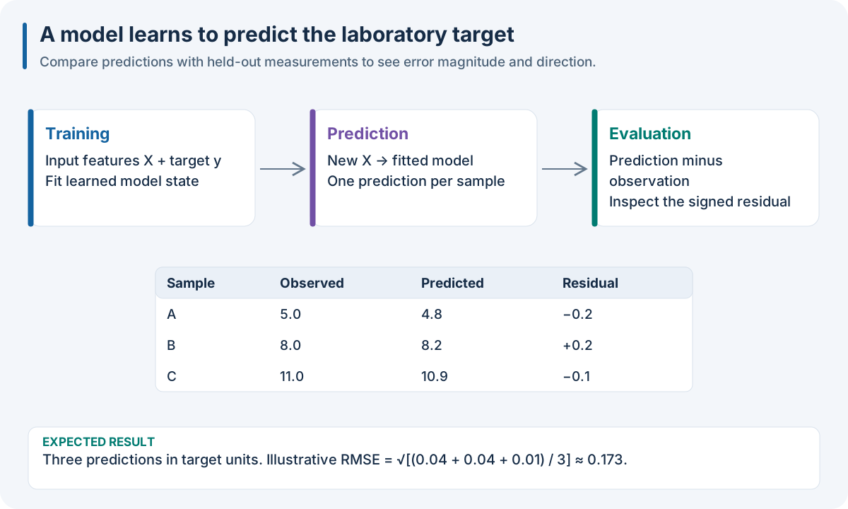
Educational workflow result; read the accompanying explanation for scope and interpretation.
An estimator learns state from X and y, predicts future rows using that state, and returns values which the target-processing node can map back to original units. The exported predictor also needs its preceding preprocessing. Model coefficients alone do not encode MSC references, selected channels or units.
PLS variants. Standard PLS creates supervised latent components. SIMPLS and IKPLS provide alternative algorithms, not new targets or independent evaluation protocols. RobustPLS reduces outlier influence; RecursivePLS introduces forgetting for sequential updates. SparsePLS constrains loading support and IntervalPLS searches contiguous bands. OPLS separates predictive and orthogonal variation, while KOPLS extends that separation in kernel space. Use the smallest adequate component count and inspect fold-to-fold stability. The number must be valid in every training fold, including internal CV.
Nonlinearity and locality. KernelPLS/KPLS/NLPLS are related public names
for kernel PLS, not three independent algorithm families. Kernel gamma,
degree and regularization assumptions influence the geometry. OKLMPLS uses a
featurizer, FCKPLS uses fractional convolution features, and LWPLS fits a
query-dependent local calibration. Local prediction can be substantially more
expensive than a single global matrix multiplication. Check the fitted
artifact’s supported consumer profile before deploying such an estimator.
Multiblock and multimodal inputs. MBPLS organizes feature blocks; typed multimodal adapters retain source and tensor structure through their declared contracts. Early feature fusion, multiblock estimation and late prediction fusion have different semantics. A model accepting a list of blocks does not automatically support every image, sequence or missing-source schema. See 4. Describe your measurements and align your sources and Public execution matrix.
Adaptive operator banks. AOM/POP families learn preprocessing alongside latent components. AOM-Ridge variants search regularized calibrations; AutoSelector chooses a candidate while Blender combines candidates. FastAOM screens chain candidates to reduce search cost. Internal tuning is additional to the workflow’s outer evaluation. Forward independent-unit/group-aware folds where supported, and preserve the bank and chosen state in export.
Stacking and residual learning. MetaModel consumes prior model
predictions selected by its configuration; selection scope and coverage
determine which rows are usable. A meta-model trained on in-sample predictions
can learn unrealistically small residuals. Use out-of-fold predictions for
training its input. A residual learner adds a correction to a base model;
its exact base/learner constructor contract is documented in
residual: learn an additive correction. See merge: decide what to bring back together for prediction fusion.
Interpret a component sweep
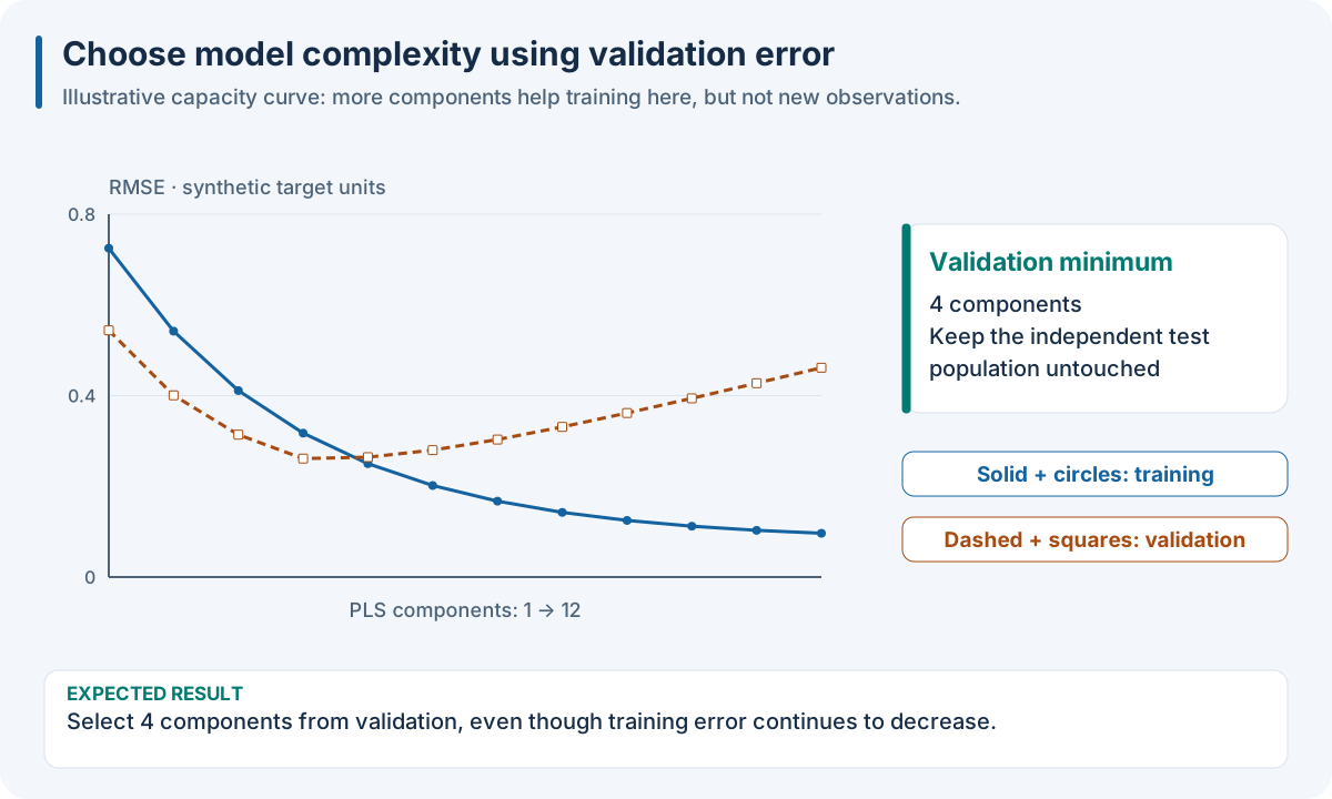
A synthetic teaching curve: select four components from validation rather than the smallest training error. These values are not a product benchmark.
The search changes the estimator’s capacity. Every candidate needs its own fitted preprocessing and model for each training fold. Refit the selected recipe on the development population only after selection. Use untouched test rows to estimate performance; report that score separately from the score which selected the recipe. Prediction intervals require additional calibration evidence, not simply a larger component count.
{
  "pipeline": [
    "nirs4all.operators.transforms.scalers.StandardNormalVariate",
    {
      "class": "sklearn.model_selection._split.KFold",
      "params": {
        "shuffle": true,
        "random_state": 42
      }
    },
    {
      "_or_": [
        {
          "model": "sklearn.cross_decomposition._pls.PLSRegression"
        },
        {
          "model": {
            "class": "sklearn.cross_decomposition._pls.PLSRegression",
            "params": {
              "n_components": 4
            }
          }
        },
        {
          "model": {
            "class": "sklearn.cross_decomposition._pls.PLSRegression",
            "params": {
              "n_components": 6
            }
          }
        }
      ]
    }
  ]
}
pipeline:
- nirs4all.operators.transforms.scalers.StandardNormalVariate
- class: sklearn.model_selection._split.KFold
  params:
    shuffle: true
    random_state: 42
- _or_:
  - model: sklearn.cross_decomposition._pls.PLSRegression
  - model:
      class: sklearn.cross_decomposition._pls.PLSRegression
      params:
        n_components: 4
  - model:
      class: sklearn.cross_decomposition._pls.PLSRegression
      params:
        n_components: 6
from sklearn.cross_decomposition import PLSRegression
from sklearn.model_selection import KFold
from nirs4all.operators.transforms import SNV

# Python SDK recipe definition: three alternative fitted calibrations.
pipeline = [
    SNV(),
    KFold(n_splits=5, shuffle=True, random_state=42),
    {"_or_": [
        {"model": PLSRegression(n_components=2)},
        {"model": PLSRegression(n_components=4)},
        {"model": PLSRegression(n_components=6)},
    ]},
]
For exact generator placement and execution, use the examples in
Generators: turn an experiment plan into concrete recipes and U04_pls_variants.py. The native catalog uses
native IDs and parameter contracts rather than sklearn import paths.
More models than this spectroscopy shortlist
The SDK also routes compatible sklearn estimators and installed neural
framework models. A discoverable class is not necessarily appropriate for the
task: for example, a classifier needs categorical targets, a count model has
domain constraints, and a supervised feature selector needs training-only y.
Inspect the constructor and fit/predict contract under API Reference.
U01_multi_model.py, U02_hyperparameter_tuning.py,
U03_stacking_ensembles.py and U07_aom_panoply.py connect those APIs to
full pipelines. Missing optional dependencies should be resolved before a run;
they are not a reason to silently switch execution engines.
Typed multimodal estimators
MultimodalRegressor(transformers, model, ...) and
MultimodalClassifier(transformers, model, ...) fit private clones of an
ordered mapping of source encoders and a prediction head. Each source keeps
its original tensor or table representation until its encoder returns a
numeric matrix. fusion="early" concatenates those matrices;
fusion="intermediate" passes a list to a compatible head. Intermediate
fusion therefore requires a model that accepts blocks, rather than an
ordinary estimator expecting a single 2-D array.
The spectral encoder and image encoder receive different shapes and produce row-aligned numeric features. Early fusion joins those columns before the Ridge head. The encoders and head are all fitted inside the supplied training population; flattening inside TensorPCA does not change sample identity.
TensorPCA(n_components=None, whiten=False, random_state=None) learns a PCA
basis after flattening the non-sample tensor dimensions. It records the exact
input shape and rejects changed image dimensions at prediction. It accepts
fixed-shape images or time tensors, not arbitrary ragged arrays. Its basis
depends on training data even though it does not use y.
Here is a standalone encoder/head experiment with synthetic, complete data. It demonstrates the estimator contract. Use the DAG workflow to add folds, evaluation and persistence; direct fitting is not a validation protocol.
import numpy as np
from sklearn.linear_model import Ridge
from nirs4all.operators.models import MultimodalRegressor, TensorPCA
from nirs4all.operators.transforms import SNV

rng = np.random.default_rng(42)
spectra = rng.normal(size=(30, 21))
images = rng.normal(size=(30, 4, 4))
y = spectra[:, 3] + images.mean(axis=(1, 2))
model = MultimodalRegressor(
    transformers={"nir": SNV(), "image": TensorPCA(n_components=3)},
    model=Ridge(alpha=1.0), fusion="early",
)
model.fit([spectra[:24], images[:24]], y[:24])
predictions = model.predict([spectra[24:], images[24:]])
assert predictions.shape == (6,)
assert model.source_names_ == ("nir", "image")
Contract |
Meaning |
|---|---|
Source order |
Input blocks follow insertion order of |
|
Nonnegative factors multiply encoded source columns; zero is an ablation, not a missing-source declaration |
|
Every source must be present |
|
Fit encoders only on present rows, use zero encoded features for absence, and append a presence column per source |
|
Boolean vectors aligned to rows; True means the source is present |
Regression |
One joint model with every target cell observed |
Regression |
A separate complete encoder/head chain for each target’s observed rows; no target imputation |
|
Boolean array with exactly y’s shape; True means observed |
|
A closed, qualified portable Methods multimodal profile; explicit IO source schemas are needed for direct fit |
Nested parameters such as transformers__image__n_components,
model__alpha and source_weights__image expose encoder/head/weight tuning.
Do not change source order or representation between training and prediction.
See U07_multimodal.py, U08_multimodal_targets.py,
U09_multimodal_missing_sources.py, U10_multimodal_late_tuning.py and
Public execution matrix for supported workflow profiles.
Late fusion uses source-specific models and OOF evidence; it is a different
workflow from choosing fusion="intermediate" on this estimator.
Principal component regression
PCR(n_components=10) fits PCA on X and ordinary least squares on the
retained scores. It is a useful unsupervised-representation baseline against
PLS: directions of largest X variance may not be the directions most useful
for predicting y. Fit both PCA and regression inside each training fold,
search component count using validation, and retain both fitted objects.