residual: learn an additive correction

Use residual learning when a strong first model explains the main relation, but a second model might explain a systematic remaining error. The second learner predicts target minus base prediction, rather than the original target.

If the base predicts 10, the correction learner predicts +2, the gate is 1 and lam=0.5, the combined prediction is 10 + 0.5 × 1 × 2 = 11. With lam=0, the result is exactly the base prediction. Correction is useful only if it improves independent validation.

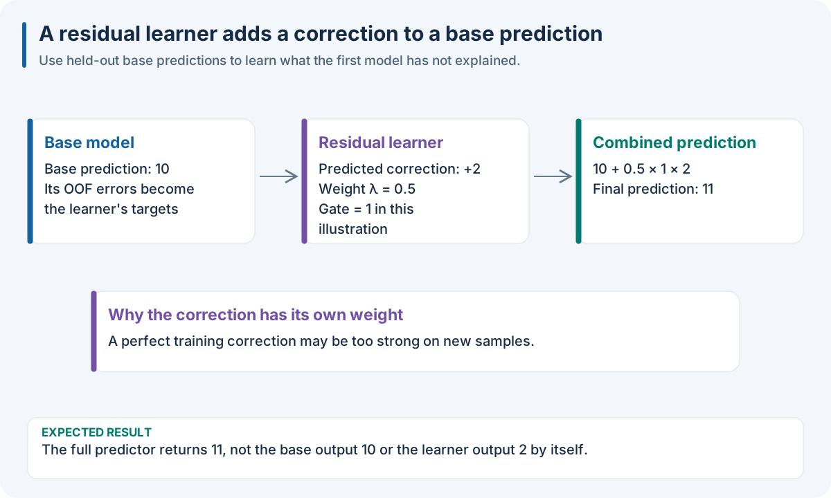
Educational additive correction. Both learners must use the same sample identities and target scale.

Worked recipe

Download dataset.json from 1. Run your first complete experiment. The JSON/YAML tabs define SDK pipeline files; the Python tab defines pipeline. The execution box below loads the same observations and runs the recipe.

JSON

{
  "pipeline": [
    {
      "split": {
        "class": "sklearn.model_selection.KFold",
        "params": {
          "n_splits": 3,
          "shuffle": true,
          "random_state": 42
        }
      }
    },
    {
      "residual": {
        "class": "nirs4all.operators.models.ResidualModel",
        "params": {
          "base": {
            "class": "sklearn.cross_decomposition.PLSRegression",
            "params": {
              "n_components": 2
            }
          },
          "learner": {
            "class": "sklearn.ensemble.RandomForestRegressor",
            "params": {
              "n_estimators": 100,
              "random_state": 42
            }
          },
          "lam": 0.5,
          "gate": false
        }
      }
    }
  ]
}

YAML

pipeline:
- split:
    class: sklearn.model_selection.KFold
    params:
      n_splits: 3
      shuffle: true
      random_state: 42
- residual:
    class: nirs4all.operators.models.ResidualModel
    params:
      base:
        class: sklearn.cross_decomposition.PLSRegression
        params:
          n_components: 2
      learner:
        class: sklearn.ensemble.RandomForestRegressor
        params:
          n_estimators: 100
          random_state: 42
      lam: 0.5
      gate: false

Python

from sklearn.cross_decomposition import PLSRegression
from sklearn.ensemble import RandomForestRegressor
from sklearn.model_selection import KFold
from nirs4all.operators.models import ResidualModel

pipeline = [
    KFold(n_splits=3, shuffle=True, random_state=42),
    {"residual": ResidualModel(
        base=PLSRegression(n_components=2),
        learner=RandomForestRegressor(n_estimators=100, random_state=42),
        lam=0.5, gate=False,
    )},
]

JSON/YAML files and Python objects here use the Python SDK. The finite R/Octave/browser pipeline facade does not accept these SDK controller keywords and Python import paths. See 10. Run the same recipe in your language for native recipes in those hosts. Equivalent local plotting or filtering does not add the SDK node’s identity, fitting-scope or export behavior.

Choices and controls

Constructor field	Meaning	Default
base	First-stage learner	Required
learner	Learner for residual targets	Required
lam	Correction multiplier	1.0
gate	"auto", a fixed scalar, or False for unit gate	"auto"
rli_threshold	Threshold for automatic abstention	0.0
train_params	Fit options forwarded to the residual learner	None
finetune_space	Search options forwarded to the residual learner	None

The public constructor names are base and learner. base_model and residual_model are not accepted aliases. You can also use a ResidualModel under model where its controller dispatch is supported.

Expected result: one combined prediction per sample/target. The residual targets use the base’s out-of-fold predictions, meaning each base prediction was produced without fitting on that sample. This protects against artificially tiny residuals from an overfit base.

Try it: compare lam=0 and lam=0.5 using identical folds. Which target regions benefit from correction? Does the learner merely chase noise?

Common mistake: reading gate=False as disabling the residual learner. It selects a unit gate; lam=0 gives the base-only check.

Learn the part the base learner misses

The combined prediction is base(X) + lam * gate * learner(X). The base provides a first explanation of the target; the learner predicts what remains. Using the base’s training predictions for residuals would make the residuals artificially small for an overfitted base, so the workflow uses out-of-fold predictions.

Constructor parameter	Meaning	Default
base	First-stage model	Required
learner	Model trained on residual targets	Required
lam	Scalar multiplier of the correction	1.0
gate	Automatic fitted gate, fixed scalar, or False for unit gate	"auto"
rli_threshold	Threshold for automatic gate abstention	0.0
train_params	Fit arguments forwarded to the learner	None
finetune_space	Search configuration forwarded to the learner	None

For the legacy controller, the automatic gate uses the OOF residual/prediction vectors, clips its least-squares weight to [0, 1], and sets it to zero if residual learnability is too low. gate=False means a unit gate, not “disable the learner”; use lam=0 when checking the base-only numerical result.

Specify folds explicitly. The base and learner must share sample identity and target scale; independently reshaping or filtering one vector breaks the residual subtraction. A complete residual evaluation also needs to protect upstream preprocessing and model selection. The legacy residual controller’s broad framework dispatch does not imply that every combination is portable; DAG-ML has separate capacity, numeric, composition and archive checks.

The constructor names are base and learner. base_model and residual_model are not accepted constructor aliases. The tracked D08 composition tutorial demonstrates source-specific multimodal preprocessing, residual fitting, export and replay. Additional executable evidence is in public-syntax integration tests, including DAG-ML export/predict and explicit legacy execution. See Public execution matrix for the broader execution contract.

Run the recipe on the downloadable observations

Install the full Python SDK as described in 1. Run your first complete experiment, execute the Python tab in the Worked recipe section to define pipeline, then run this box. It reads the first experiment’s complete single-source dense fixture into its numeric SDK arrays. The fixture has 12 rows × 7 features, one target and training rows only; its figures’ small numeric examples explain the mechanisms independently of the fixture’s fitted predictions.

Python SDK execution

import json
from pathlib import Path
import numpy as np
import nirs4all
from sklearn.model_selection import KFold
from sklearn.cross_decomposition import PLSRegression

# Download dataset.json, then run the Python tab in the Worked recipe section.
observations = json.loads(Path("dataset.json").read_text())["dataset"]
X = np.asarray(observations["sources"][0]["array"]["values"], dtype=float)
y = np.asarray(observations["y"]["values"], dtype=float)
complete_pipeline = pipeline
result = nirs4all.run(
    complete_pipeline, (X, y), engine="dag-ml",
    workspace_path="workspace-node-example", verbose=0,
)
validation = result.predictions.filter_predictions(partition="val")
print(validation[0]["val_score"])

Expected: a completed three-fold calibration, finite validation scores, and stored results in workspace-node-example. With no independent test rows in this teaching fixture, inspect val_score; a final-test convenience score may be absent/NaN. The chart recipe also saves its diagnostics. Keep your own study’s sample/source identities and group metadata when replacing this simple fixture.