Transforms Reference
A transform changes the features presented to a model. Choose it from a measurement question, then verify that useful signal survives. For example, scatter correction removes gain/offset differences; smoothing suppresses rapid oscillations; derivatives emphasize slopes; resampling changes where spectra are evaluated.
Choose a transform by the effect you want to remove
Read Preprocessing: change what the model sees for the worked result figure, expected dimensions and exercises. Choose a family below to compare the enumerated operators.
Same worked recipe in JSON, YAML and Python
{
  "pipeline": [
    {
      "class": "nirs4all.operators.transforms.StandardNormalVariate"
    }
  ]
}
pipeline:
- class: nirs4all.operators.transforms.StandardNormalVariate
from nirs4all.operators.transforms import SNV

pipeline = [SNV()]
These are Python SDK operators. Native R/Octave/WASM recipes use their own method IDs and facade; see 10. Run the same recipe in your language.
Scatter Correction and Normalization
Class |
Key Parameters |
Description |
|---|---|---|
|
|
Row-wise centering and scaling to remove scatter effects |
|
|
Per-sample local normalization with a sliding window along features |
|
|
Robust centering (median) and scaling (MAD) per sample |
|
|
Corrects scatter by regressing each spectrum against the mean reference |
|
|
MSC extended with polynomial terms to model chemical and physical scatter |
|
|
Normalizes each spectrum by its total area; method: |
|
|
Range normalization or linalg normalization when range is |
|
(none) |
Column-wise min-max scaling to [0, 1] |
Smoothing
Class |
Key Parameters |
Description |
|---|---|---|
|
|
Savitzky-Golay polynomial smoothing and optional derivative computation |
|
|
1D Gaussian filter using |
|
|
Multi-level wavelet decomposition with thresholding for denoising |
Derivatives
Class |
Key Parameters |
Description |
|---|---|---|
|
|
First numerical derivative using |
|
|
Second numerical derivative using |
|
|
Gap derivative with segment smoothing (Norris-Williams method) |
|
|
Nth-order wavelength derivative; |
Baseline Correction
Simple
Class |
Key Parameters |
Description |
|---|---|---|
|
(none) |
Removes the column-wise mean baseline from each spectrum |
|
|
Removes linear trend using |
pybaselines Wrappers
All baseline correction classes below wrap the pybaselines library. They share a common interface via PyBaselineCorrection.
Class |
Key Parameters |
Description |
|---|---|---|
|
|
General wrapper for any pybaselines method |
|
|
Asymmetric Least Squares baseline correction |
|
|
Adaptive Iteratively Reweighted Penalized Least Squares |
|
|
Asymmetrically Reweighted Penalized Least Squares |
|
|
Improved Modified Polynomial baseline correction |
|
|
Modified Polynomial baseline correction |
|
|
Statistics-sensitive Non-linear Iterative Peak-clipping |
|
|
Morphological rolling ball baseline estimation |
|
|
Improved Asymmetric Least Squares |
|
|
Baseline Estimation And Denoising with Sparsity |
Orthogonalization
Class |
Key Parameters |
Description |
|---|---|---|
|
|
Orthogonal Signal Correction – removes Y-orthogonal variation from X (supervised, requires y) |
|
|
External Parameter Orthogonalization – removes variation correlated with external parameters (e.g., temperature) |
Note
OSC requires y during fit(). EPO requires external parameters d during fit(), not y.
Signal Conversion
Class |
Key Parameters |
Description |
|---|---|---|
|
|
Converts reflectance to absorbance via Beer-Lambert law: A = -log10(R) |
|
|
Converts reflectance or transmittance to absorbance; supports percent inputs |
|
|
Converts absorbance back to reflectance or transmittance via 10^(-A) |
|
|
General-purpose converter that auto-determines the conversion path |
|
|
Kubelka-Munk transformation for diffuse reflectance: F(R) = (1-R)^2 / (2R) |
|
|
Elementwise logarithm with automatic handling of zeros/negatives |
|
(none) |
Divides by 100 to convert percentage values to fractional [0, 1] range |
|
(none) |
Multiplies by 100 to convert fractional values to percentage range |
Wavelet Transforms and Feature Extraction
Class |
Key Parameters |
Description |
|---|---|---|
|
|
Single-level Discrete Wavelet Transform |
|
(none) |
Shortcut for |
|
|
Extracts statistical features from wavelet decomposition at multiple scales |
|
|
Multi-scale PCA on wavelet coefficients for compact multi-resolution representation |
|
|
Multi-scale SVD on wavelet coefficients (no centering, works for sparse data) |
Feature Selection
Class |
Key Parameters |
Description |
|---|---|---|
|
|
Competitive Adaptive Reweighted Sampling for wavelength selection (requires y) |
|
|
Monte-Carlo Uninformative Variable Elimination (requires y) |
|
|
PCA with flexible specification: int for count, float in (0,1) for variance ratio |
|
|
Truncated SVD with flexible specification: int for count, float in (0,1) for variance ratio |
Resampling and Cropping
Class |
Key Parameters |
Description |
|---|---|---|
|
|
Resamples spectral data to a new wavelength grid using scipy interpolation |
|
|
Crops features by index range [start:end] |
|
|
Resamples each spectrum to a fixed number of points via linear interpolation |
|
|
Flattens 3D (samples, preprocessings, features) to 2D by concatenating preprocessing views |
Target Transforms
Class |
Key Parameters |
Description |
|---|---|---|
|
(imported from targets) |
Discretizes continuous targets into integer bins |
|
(imported from targets) |
Discretizes targets based on value ranges |
See Also
Augmentation Operators Reference – Data augmentation operators
Pipeline Keywords Reference – Pipeline keyword syntax reference
Operator catalog: choose a job, then inspect the method – Full operator catalog
How to interpret and combine the families
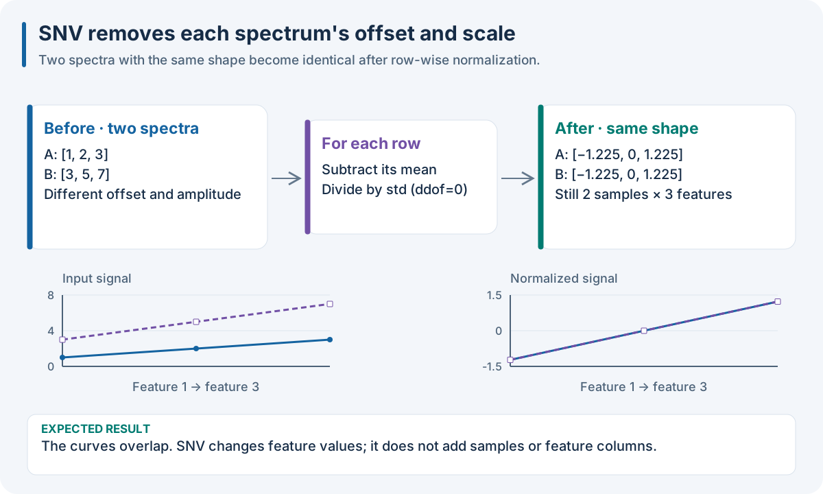
Educational SNV example: [1, 2, 3] and [3, 5, 7] both become approximately
[-1.225, 0, 1.225]. The mechanism removes gain/offset, not sample identity.
Scatter correction. StandardNormalVariate uses each row’s mean and
standard deviation; it does not estimate the population mean spectrum.
LocalStandardNormalVariate uses local windows and can alter peak contrast
at window boundaries. RobustStandardNormalVariate substitutes median and
MAD, reducing the influence of spikes on normalization. MSC learns the mean
training spectrum and corrects each row using a fitted offset and slope.
EMSC extends that regression with polynomial nuisance terms. The current
MSC scale argument is retained for API compatibility and does not change
the raw-spectrum reference calculation. Fit its reference on training rows.
Area normalization compares relative spectral contributions; it can discard
absolute intensity that was useful for predicting concentration.
Smoothing and derivatives. Savitzky–Golay fits a local polynomial to a
window. Increase window_length to suppress more noise at the cost of
blurring narrow peaks; polyorder must be smaller than the window length.
Set deriv=0 for smoothing and deriv=1 or 2 for smoothed derivatives.
delta is the grid spacing and controls derivative units. The usual choice
is an odd window no longer than the spectrum. Gaussian filtering spreads
each point over its neighbors; sigma controls that scale. First/second
derivatives differentiate along the spectral axis, while Norris–Williams
adds segment averaging and a gap. Wavelet denoising thresholds detail
coefficients; its level, boundary mode and threshold can change edge peaks.
Inspect those boundaries before comparing validation scores.
Baseline correction. Detrend removes a linear trend. AsLS and IAsLS
balance smoothness (lam) against asymmetric treatment of peaks (p);
AirPLS and ArPLS adapt weights iteratively. ModPoly and IModPoly use
polynomial baselines; SNIP iteratively clips peaks, RollingBall uses a
morphological envelope, and BEADS combines sparse signal and baseline
estimation. These methods encode different beliefs about the baseline.
Do not choose a method solely because it makes a spectrum visually flat:
broad chemical peaks may also be removed. Optional pybaselines is needed
for its wrappers.
Orthogonalization. OSC learns directions in X that are orthogonal to y.
It is supervised even though it appears before the model. EPO learns a
spectral interference subspace from external parameters d, such as
temperature; d is not the prediction target. EPO’s fitted projection can
then transform future spectra without requiring d. Both learn state
inside training folds. See U05_orthogonalization.py for external-parameter
binding in a full workflow.
Physical conversions. Reflectance-to-absorbance computes -log10(R) for
fractional reflectance; percent reflectance requires dividing by 100 first
or declaring the appropriate source type. FromAbsorbance applies the
inverse exponential. SignalTypeConverter selects the conversion from its
declared source and target types; it does not establish those types from
chemistry. Kubelka–Munk computes (1-R)^2/(2R) for diffuse reflectance.
LogTransform is a general numerical logarithm with offset rules, which need
not have a physical absorbance interpretation. Keep units and signal type
with the source schema, especially across language boundaries.
Representation and selection. Wavelet/Haar return coefficients; WaveletFeatures summarizes coefficients at multiple scales. WaveletPCA and WaveletSVD learn reductions at each scale, so their fitted bases must be reused at prediction. FlexiblePCA centers its input and FlexibleSVD offers a truncated SVD representation. CARS and MCUVE use y to select wavelengths; their internal selection must not see outer validation targets. Cropping removes indexed channels, resampling changes the grid, and flattening joins preprocessing views. Each changes how downstream feature positions should be interpreted. An index crop does not imply a particular physical wavelength range unless the schema establishes that mapping.
A complete, small transformation experiment
This standalone Python example exposes fitted state explicitly. It creates training and future rows, fits MSC on training only, then reuses its reference. It is a numerical experiment rather than a cross-validation pipeline.
import numpy as np
from nirs4all.operators.transforms import MSC, SNV, SavitzkyGolay

wavelengths = np.linspace(1000, 2200, 241)  # 5 nm spacing
peak = np.exp(-((wavelengths - 1450) / 100) ** 2)
X_train = np.stack([peak, 1.2 * peak + 0.1, 0.8 * peak - 0.05])
X_future = np.stack([1.1 * peak + 0.08])

msc = MSC().fit(X_train)
corrected_train = msc.transform(X_train)
corrected_future = msc.transform(X_future)
assert corrected_future.shape == (1, 241)

snv = SNV().fit_transform(X_train)
assert np.allclose(snv.mean(axis=1), 0, atol=1e-12)
derivative = SavitzkyGolay(
    window_length=11, polyorder=3, deriv=1, delta=5.0
).fit_transform(X_train)
assert derivative.shape == X_train.shape
For workflow-level fit scope use Preprocessing: change what the model sees, not manual prefitting on the whole dataset. A Python SDK serialized preprocessing node can be written as follows; this import-path form is not a portable native ID:
preprocessing:
  class: nirs4all.operators.transforms.SavitzkyGolay
  params:
    window_length: 11
    polyorder: 3
    deriv: 1
    delta: 5.0
Learning exercises and exact APIs
Run U01_preprocessing_basics.py to compare transformations, then
U04_signal_conversion.py to inspect declared units and
U06_wavelet_denoise.py to inspect scale and boundary behavior. Compare one
factor at a time on the same folds. Preserve the fitted transform and feature
schema with the final model.
The API Reference tree contains per-class constructor and method
documentation under nirs4all.operators.transforms. The native operator IDs
and binding availability are separate contracts: consult
0. Choose the tools for your language before translating an import path to another host.
Ragged temporal encoding: SequenceSummary
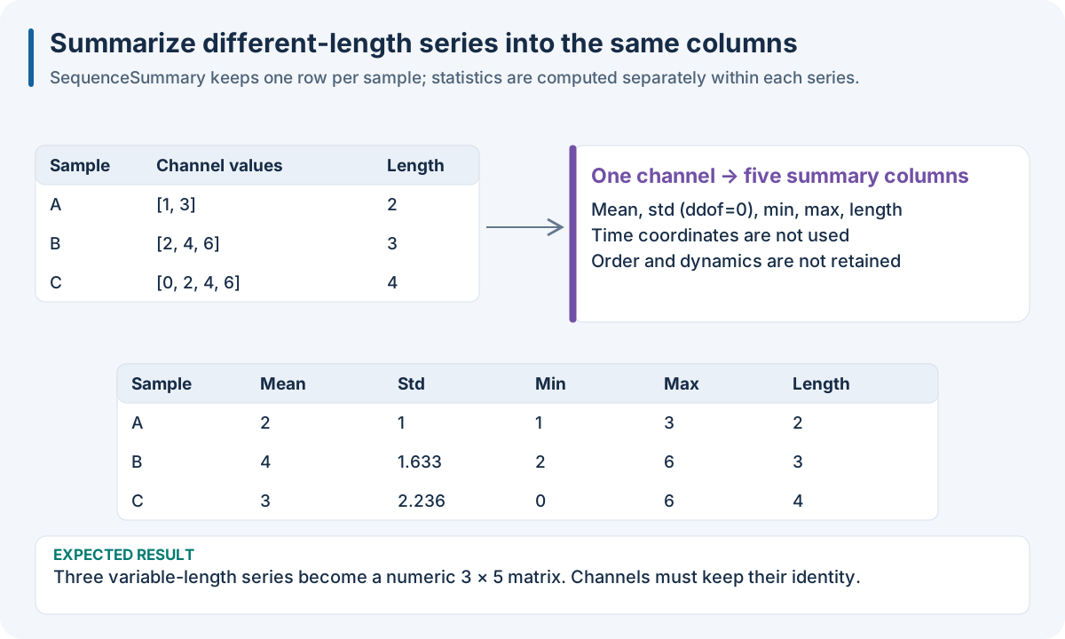
Educational one-channel example. Sequences of length 2, 3 and 4 keep their sample identity while becoming a matrix with three rows and five columns. Values are described below.
Observed sequence |
Mean |
Population SD |
Minimum |
Maximum |
Length |
|---|---|---|---|---|---|
|
2 |
1 |
1 |
3 |
2 |
|
4 |
1.633 |
2 |
6 |
3 |
|
3 |
2.236 |
0 |
6 |
4 |
The summary uses equally weighted observations. It ignores time-coordinate spacing and loses the ordering of measurements. With several channels, summaries are constructed per channel and channel identity must remain fixed. The observation-count feature is optional; it is not elapsed time.
SequenceSummary accepts an IO RaggedSeriesBatch: one variable-length
multichannel series per sample. It computes an ordered subset of mean,
std, min and max for each channel, optionally appending observation count.
For two channels, four statistics and include_length=True, output width
is 2 × 4 + 1 = 9, regardless of individual series lengths. Columns are
ordered by channel, then statistic; length is last. Standard deviation uses
ddof=0.
Each sample is summarized independently into the same column contract. Sequence lengths are allowed to differ; channel identities must stay fixed. The optional length feature describes measurement count, not elapsed time.
The encoder deliberately ignores time coordinates and weights observations equally. Therefore an arithmetic mean is not a time-weighted mean for irregular sampling; order and dynamics are lost. Use it when aggregate behavior is a plausible representation, and compare against an appropriate temporal representation when dynamics matter.
channel_names supplies stable names. min_observations=1 accepts singleton
series; a larger value makes an explicit applicability rule.
channel_bounds supplies inclusive finite domain limits per channel and is
not inferred from held-out observations. Empty series and nonfinite observed
values are refused. A missing modality must be handled by its presence policy
before reaching the encoder; do not pad it with fake measurements.
Fit records the channel contract, not training values or lengths. Run
U12_multimodal_ragged_series.py, U13_multimodal_late_missing_sources.py
and 4. Describe your measurements and align your sources for workflow, missingness and domain
examples. Availability of this Python encoder does not imply an identical
ragged runtime profile in every binding.
Fixed convolution features: FCKStaticTransformer
FCKStaticTransformer applies a constructor-defined bank of normalized
fractional convolution filters along wavelengths. The defaults combine four
orders, two scales and two kernel sizes into 16 filters. With flattening,
(n, p) becomes (n, 16p); flatten=False retains (n, 16, p).
alphas, scales, kernel_sizes and sigma define the bank;
mode defines boundary handling. It does not learn filters from y or the
training population, but selecting its hyperparameters still requires
training/validation separation. Large banks increase memory and model
complexity. Compare its added representations against a simple derivative
baseline rather than treating more columns as additional independent evidence.