`model`: turn features into predictions

A model learns from examples with known targets, then predicts the target of an unseen sample. Use regression for a measurement such as protein concentration; use classification for a category such as healthy/diseased.

For one regression target, 3 samples × 21 wavelengths produce 3 predictions × 1 target. Illustrative targets [5, 8, 11] and predictions [4.8, 8.2, 10.9] have errors [-0.2, +0.2, -0.1] and RMSE 0.173 target units. These values explain the score; they are not promised outputs from the recipe.

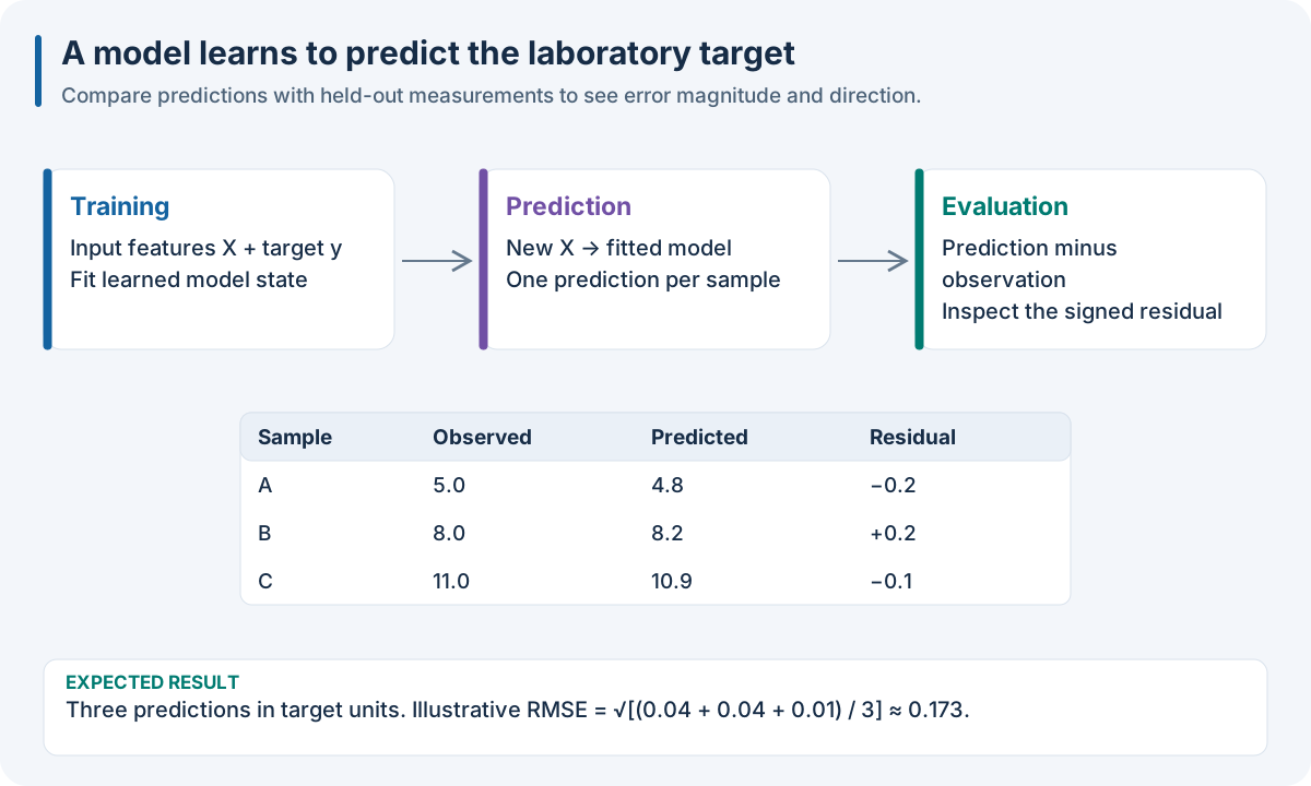
Educational prediction example. Prediction count and target units are preserved.

Worked recipe

Download dataset.json from 1. Run your first complete experiment. JSON/YAML can be saved as SDK pipeline files; the Python tab defines pipeline. The execution box below loads those same observations and runs this SDK recipe.

JSON

{
  "pipeline": [
    {
      "class": "nirs4all.operators.transforms.StandardNormalVariate"
    },
    {
      "split": {
        "class": "sklearn.model_selection.KFold",
        "params": {
          "n_splits": 3,
          "shuffle": true,
          "random_state": 42
        }
      }
    },
    {
      "model": {
        "class": "sklearn.cross_decomposition.PLSRegression",
        "params": {
          "n_components": 2
        }
      },
      "name": "PLS-2"
    }
  ]
}

YAML

pipeline:
- class: nirs4all.operators.transforms.StandardNormalVariate
- split:
    class: sklearn.model_selection.KFold
    params:
      n_splits: 3
      shuffle: true
      random_state: 42
- model:
    class: sklearn.cross_decomposition.PLSRegression
    params:
      n_components: 2
  name: PLS-2

Python

from nirs4all.operators.transforms import SNV
from sklearn.model_selection import KFold
from sklearn.cross_decomposition import PLSRegression

pipeline = [
    SNV(), KFold(n_splits=3, shuffle=True, random_state=42),
    {"model": PLSRegression(n_components=2), "name": "PLS-2"},
]

The JSON/YAML tabs define SDK recipes; the Python tab builds the same recipe with objects. These examples use Python SDK operators. The R, Octave and browser/WASM finite pipeline facade uses native method IDs, not Python import paths. Use 10. Run the same recipe in your language for its actual binding calls and 0. Choose the tools for your language to choose the runtime.

Choices and controls

Field/form	Responsibility	Example
`model` with serialized `class`/`params`	Instantiate the learner	PLS with two components
`model` with a Python object	Use a configured estimator	Interactive recipe
Bare Python estimator	Automatically detect an object with `predict()`	Short Python pipelines
Constructor `params`	Configure scientific/model choices	Components, regularization, kernel
`train_params` beside `model`	Supported fitting arguments	Neural epochs or batch size
`finetune_params` beside `model`	Search inside the model fitting scope	See Hyperparameter Tuning
`name`	Human-readable result label	`PLS-2`

Learning question	Starting families	Main decision
Transparent calibration baseline	PLS, Ridge, PCR	Components or regularization
Categorize samples	`PLSDA`, sklearn classifiers	Labels, class balance, probabilities
Remove target-unrelated variation	`OPLS`, `OPLSDA`	Predictive and orthogonal components
Nonlinear relation	Kernel PLS, SVR, tree ensembles	Complexity and available sample size
Aligned multiple blocks	`MBPLS`, `MultimodalRegressor`	Source schema and fusion strategy
Learn preprocessing with calibration	AOM/POP families	Operator bank and internal CV
Combine predictions	`MetaModel`, `ResidualModel`	Out-of-fold evidence and composition
Large structured inputs	Installed Torch/TF/JAX models	Architecture, training data, deployment runtime

Expected result: a prediction for every target of every submitted row. For classification, distinguish labels from probabilities. Export the whole predictor with preprocessing and target inversion.

Try it: compare 1, 2 and 4 PLS components using identical folds. Does the best validation recipe also have the smallest training error?

Common mistake: choosing capacity using the final test score. That turns the test population into model-selection data. Also keep components below the capacity of the smallest training fold.

Reading the training lifecycle

Cross-validation estimates behavior on observations held out from a fit. Refit prepares the selected configuration for use on all permitted training observations. The final test partition is reserved for evaluation; selecting a learner or its hyperparameters because it performs best on that test set changes the meaning of the reported score.

Field	Responsibility	Example
`model.params`	Constructor configuration	`n_components: 5` or `alpha: 1.0`
`train_params`	Framework-specific fitting options	Neural training epochs or batch size
`finetune_params`	Search inside a model training scope	Model-local hyperparameter optimization
`refit_params`	Refit-specific policy where supported	See the engine-specific refit reference
`name`	Result/trace label	`PLS-5`

These fields are distinct contracts; support depends on the controller and engine. A Python sklearn estimator is a host learner. A native Methods PLS operator may solve the same task but has different serialization, export and runtime support. Installing a neural framework does not make its model portable to WASM.

Capacity and output checks

Keep n_components below the rank/size available in the smallest fitting fold. Start with a small value and inspect the validation curve before increasing capacity. For classifiers, verify label encoding and whether the downstream operation requires class labels, probabilities or scores. For multi-target regression, confirm that the learner and prediction artifact preserve all target columns.

A sequence of two model nodes records/evaluates successive models on the active features; it is not automatically a chain in which the second learns from the first model’s predictions. Use merge: decide what to bring back together or an explicit meta-model for stacking and residual: learn an additive correction for additive correction.

Worked source: stacking configuration. See 7. Read the result and keep a useful experiment record to select and interpret results and 8. Save a predictor and use it on new observations for export/replay contracts.

A portable model recipe in all six representations

This alternative uses feature standardization followed by Ridge, rather than the SDK PLS example. Standardization learns each feature’s mean and scale from the training rows; Ridge shrinks its coefficients by alpha=1. This operation is available through the finite native facade in every host below. The exact recipe syntax differs from SDK import-path serialization.

Use dataset.json from 1. Run your first complete experiment. Save the JSON tab as ridge.recipe.json. YAML expresses the same mapping; parse it with your host YAML library before calling the facade. CPU hosts need the Core CLI and Methods library configured as in Move a native model or a complete experiment; the browser needs the matching WASM assets served over HTTP. This example defines one candidate; its dataset carries the validation assignment.

JSON

{
  "steps": [
    {
      "method_id": "preprocessing.scaling.standard_scale",
      "role": "transformer",
      "params": {}
    },
    {
      "method_id": "models.regularized.ridge",
      "role": "regressor",
      "params": {
        "scale_x": false
      }
    }
  ],
  "candidates": [
    {
      "alpha": 1.0
    }
  ]
}

YAML

steps:
- method_id: preprocessing.scaling.standard_scale
  role: transformer
  params: {}
- method_id: models.regularized.ridge
  role: regressor
  params:
    scale_x: false
candidates:
- alpha: 1.0

Python Core

import json
from pathlib import Path
from nirs4all_core import run_pipeline

training = json.loads(Path("dataset.json").read_text())
recipe = json.loads(Path("ridge.recipe.json").read_text())
model = run_pipeline(training, recipe)
model.export("ridge.native.json")

R native

library(nirs4all)
training <- jsonlite::fromJSON("dataset.json", simplifyVector = FALSE)
recipe <- jsonlite::fromJSON("ridge.recipe.json", simplifyVector = FALSE)
model <- nirs4all_run_pipeline(training, recipe)
nirs4all_pipeline_export(model, "ridge.native.json")

Octave / MATLAB

training = fileread('dataset.json');
recipe = fileread('ridge.recipe.json');
model = nirs4all.runPipeline(training, recipe);
model.export('ridge.native.json');

WASM browser

import {runBrowserPipeline} from 'nirs4all';

const training = await (await fetch('./dataset.json')).json();
const recipe = await (await fetch('./ridge.recipe.json')).json();
const model = await runBrowserPipeline(training, {pipeline: recipe});
localStorage.setItem('ridge-native', model.export());

Expected result: a fitted native model and its exported native JSON package. For a future matrix with m rows and one target, prediction returns m target values with their sample identities. This export is the finite native package; its filename does not make it an Archive V2 .n4a bundle. Follow 10. Run the same recipe in your language for verified reload/predict calls in the same languages.

Run the recipe on the downloadable observations

Install the full Python SDK as described in 1. Run your first complete experiment, execute the Python tab in the Worked recipe section to define pipeline, then run this box. It reads the first experiment’s complete single-source dense fixture into its numeric SDK arrays. The fixture has 12 rows × 7 features, one target and training rows only; its figures’ small numeric examples explain the mechanisms independently of the fixture’s fitted predictions.

Python SDK execution

import json
from pathlib import Path
import numpy as np
import nirs4all
from sklearn.model_selection import KFold
from sklearn.cross_decomposition import PLSRegression

# Download dataset.json, then run the Python tab in the Worked recipe section.
observations = json.loads(Path("dataset.json").read_text())["dataset"]
X = np.asarray(observations["sources"][0]["array"]["values"], dtype=float)
y = np.asarray(observations["y"]["values"], dtype=float)
complete_pipeline = pipeline
result = nirs4all.run(
    complete_pipeline, (X, y), engine="dag-ml",
    workspace_path="workspace-node-example", verbose=0,
)
validation = result.predictions.filter_predictions(partition="val")
print(validation[0]["val_score"])

Expected: a completed three-fold calibration, finite validation scores, and stored results in workspace-node-example. With no independent test rows in this teaching fixture, inspect val_score; a final-test convenience score may be absent/NaN. The chart recipe also saves its diagnostics. Keep your own study’s sample/source identities and group metadata when replacing this simple fixture.

model: turn features into predictions