tag: flag a sample and keep it

Use tagging when you want to investigate unusual observations before deciding whether they should influence calibration. A tag adds an explanation to a sample. It does not remove that sample or change its measured value.

For targets [10, 11, 12, 13, 14, 50], the IQR rule below computes Q1 = 11.25, Q3 = 13.75 and IQR = 2.5. With threshold 1.5, acceptable values span 7.5–17.5. Only the sixth target, 50, is flagged. All six rows remain available.

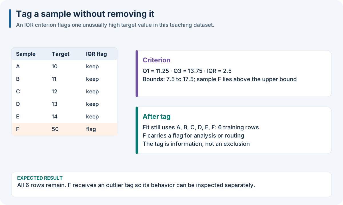
Educational IQR example using the actual filter percentile convention. Flagged means inspect, not prove invalid.

Worked recipe

Download dataset.json from 1. Run your first complete experiment. The JSON/YAML tabs define SDK pipeline files; the Python tab defines pipeline. The execution box below loads the same observations and runs the recipe.

JSON

{
  "pipeline": [
    {
      "tag": {
        "class": "nirs4all.operators.filters.YOutlierFilter",
        "params": {
          "method": "iqr",
          "threshold": 1.5,
          "tag_name": "extreme_target"
        }
      }
    }
  ]
}

YAML

pipeline:
- tag:
    class: nirs4all.operators.filters.YOutlierFilter
    params:
      method: iqr
      threshold: 1.5
      tag_name: extreme_target

Python

from nirs4all.operators.filters import YOutlierFilter

pipeline = [{"tag": YOutlierFilter(
    method="iqr", threshold=1.5, tag_name="extreme_target",
)}]

JSON/YAML files and Python objects here use the Python SDK. The finite R/Octave/browser pipeline facade does not accept these SDK controller keywords and Python import paths. See 10. Run the same recipe in your language for native recipes in those hosts. Equivalent local plotting or filtering does not add the SDK node’s identity, fitting-scope or export behavior.

Choices and controls

Form/control	Effect
tag with one filter	Add its boolean flag column
tag with a list of filters	Add separate flags for each criterion
tag with named filter mapping	Give each criterion an explicit column name
Filter tag_name	Name the flag; otherwise the exclusion reason supplies a name
YOutlierFilter	Flag extreme known target values
XOutlierFilter	Flag spectral distance/density/reconstruction anomalies
SpectralQualityFilter	Flag NaN, infinity, zeros, flatness or saturation
HighLeverageFilter	Flag unusual influential feature positions
MetadataFilter	Apply a declared rule to a metadata column

Expected result: six rows and a flag vector [false, false, false, false, false, true] for the educational example. A filter’s get_mask() uses True = keep; the stored outlier tag inverts it to True = flagged.

Try it: tag first, then report model errors separately on flagged and unflagged samples. Are the rare targets inaccurate, or merely unusual?

Common mistake: treating a rare valid concentration as a faulty measurement. Also, a YOutlierFilter cannot classify new unlabeled spectra: it needs observed y.

A tag is evidence, not a removal decision

The filter mask uses True = keep. The tag controller inverts that mask so a boolean outlier tag uses True = flagged. A tag therefore needs a clear name; a filter’s keep-mask and the stored tag do not have the same boolean meaning. Multiple filters produce separate tag columns rather than one implicit combined exclusion rule.

During training, the legacy controller fits the criterion on base training rows and tags the selected cohort. Prediction can apply persisted filter state; if that state is absent, the controller can fit on the incoming cohort. These are different thresholds and should not be conflated when interpreting deployment monitoring.

YOutlierFilter requires known targets to evaluate an observation. Use it for training diagnostics; for unlabeled prediction routes, choose a criterion that uses available spectra or metadata. A metadata route also requires that column in every prediction request. Tags preserve observations, making them useful for reporting a model’s error separately on flagged and unflagged cohorts.

Worked source: sample filtering tutorial. Filter masks and thresholds are detailed in Filters Reference.

Run the recipe on the downloadable observations

The node recipe above performs a preprocessing/diagnostic operation. The execution box adds three-fold validation and a two-component PLS learner so you can run a complete calibration. Install the full Python SDK as described in 1. Run your first complete experiment, execute the Python tab in the Worked recipe section to define pipeline, then run this box. It reads the first experiment’s complete single-source dense fixture into its numeric SDK arrays. The fixture has 12 rows × 7 features, one target and training rows only; its figures’ small numeric examples explain the mechanisms independently of the fixture’s fitted predictions.

Python SDK execution

import json
from pathlib import Path
import numpy as np
import nirs4all
from sklearn.model_selection import KFold
from sklearn.cross_decomposition import PLSRegression

# Download dataset.json, then run the Python tab in the Worked recipe section.
observations = json.loads(Path("dataset.json").read_text())["dataset"]
X = np.asarray(observations["sources"][0]["array"]["values"], dtype=float)
y = np.asarray(observations["y"]["values"], dtype=float)
complete_pipeline = [*pipeline, KFold(n_splits=3),
                     {"model": PLSRegression(n_components=2)}]
result = nirs4all.run(
    complete_pipeline, (X, y), engine="dag-ml",
    workspace_path="workspace-node-example", verbose=0,
)
validation = result.predictions.filter_predictions(partition="val")
print(validation[0]["val_score"])

Expected: a completed three-fold calibration, finite validation scores, and stored results in workspace-node-example. With no independent test rows in this teaching fixture, inspect val_score; a final-test convenience score may be absent/NaN. The chart recipe also saves its diagnostics. Keep your own study’s sample/source identities and group metadata when replacing this simple fixture.