sample_augmentation: give training examples plausible variants

Use sample augmentation when realistic measurement variation can help the model tolerate instrument noise, shifts or drift. It creates synthetic training rows that keep an origin relationship to real observations. A synthetic copy is not a new independent specimen.

Suppose one fold contains eight real training rows and four validation rows. With count: 2, create two variants per training origin: 8 originals + 16 variants = 24 fitting rows. Validation still evaluates four original rows. Future prediction adds no random copies.

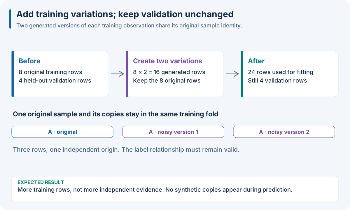
Educational fold-local augmentation. Copies retain origin IDs and target relationships; they do not increase the independent sample count.

Worked recipe

Download dataset.json from 1. Run your first complete experiment. The JSON/YAML tabs define SDK pipeline files; the Python tab defines pipeline. The execution box below loads the same observations and runs the recipe.

JSON

{
  "pipeline": [
    {
      "split": {
        "class": "sklearn.model_selection.KFold",
        "params": {
          "n_splits": 3
        }
      }
    },
    {
      "sample_augmentation": {
        "transformers": [
          {
            "class": "nirs4all.operators.augmentation.GaussianAdditiveNoise",
            "params": {
              "sigma": 0.01
            }
          }
        ],
        "count": 2,
        "selection": "random",
        "random_state": 42
      }
    },
    {
      "model": {
        "class": "sklearn.cross_decomposition.PLSRegression",
        "params": {
          "n_components": 2
        }
      }
    }
  ]
}

YAML

pipeline:
- split:
    class: sklearn.model_selection.KFold
    params:
      n_splits: 3
- sample_augmentation:
    transformers:
    - class: nirs4all.operators.augmentation.GaussianAdditiveNoise
      params:
        sigma: 0.01
    count: 2
    selection: random
    random_state: 42
- model:
    class: sklearn.cross_decomposition.PLSRegression
    params:
      n_components: 2

Python

from sklearn.model_selection import KFold
from sklearn.cross_decomposition import PLSRegression
from nirs4all.operators.augmentation import GaussianAdditiveNoise

pipeline = [
    KFold(n_splits=3),
    {"sample_augmentation": {
        "transformers": [GaussianAdditiveNoise(sigma=0.01)],
        "count": 2, "selection": "random", "random_state": 42,
    }},
    {"model": PLSRegression(n_components=2)},
]

JSON/YAML files and Python objects here use the Python SDK. The finite R/Octave/browser pipeline facade does not accept these SDK controller keywords and Python import paths. See 10. Run the same recipe in your language for native recipes in those hosts. Equivalent local plotting or filtering does not add the SDK node’s identity, fitting-scope or export behavior.

Choices and controls

Run this example with the supported DAG-ML augmentation workflow so validation rows remain outside the synthetic training population.

Control	Meaning
transformers	Candidate perturbations; at least one is required
count	Requested copies per origin in ordinary mode
selection: random	Randomly choose among the candidates
selection: all	Cycle candidates to satisfy the requested count
random_state	Reproduce selection and derive seeds for unseeded augmenters
balance: y	Balance target classes, or concentration bins for regression
balance: metadata_column	Balance a declared metadata cohort
target_size	Target count per cohort
max_factor	Limit cohort expansion by a multiplier
ref_percentage	Target fraction of the majority cohort
bins	Number of regression target bins (default 10)
binning_strategy	equal_width or quantile
bin_balancing	sample or regression value balancing
variation_scope	Sample-specific or shared-batch variation where the augmenter supports it

Choose one balancing size strategy. Ordinary count mode and balanced mode answer different questions.

For GaussianAdditiveNoise(sigma=0.01) in sample mode, noise standard deviation is 0.01 times each spectrum’s standard deviation, not an absolute absorbance 0.01. The smoothing_kernel_width can correlate neighboring noise. Explicit operator seeds take priority over the step seed.

Expected result: more training rows with the same feature width and declared target relationship. Validation/test rows and future prediction counts do not increase. Check physical plausibility in an Chart nodes: ask a concrete question of the current data comparison.

Try it: compare count=0, count=1 and count=2 using the same folds and model. Record independent origin count as well as synthetic row count.

Common mistake: generating copies, then randomly treating them as independent samples. Also, mixing two materials requires corresponding mixed targets; target-changing mixup cannot be used as a target-preserving augmenter here.

DAG-ML execution

With engine="dag-ml", augmentation trains on original and synthetic training rows. Validation and test scores still cover the original rows only. Without a cross-validator, DAG-ML fits once and reports no CV score. With a cross-validator, stateless augmenters can generate rows before splitting; balanced or data-dependent augmenters generate separate rows within each fold’s training partition and during refit. Repetition datasets retain group-aware folds.

Consecutive augmentation steps work with or without CV. Augmentation steps can also be separated by preprocessing steps. For balanced or data-dependent augmentation, each CV fold materializes its own ordered augmentation and preprocessing chain, including transformed validation spectra; refit uses the full training partition. The fitted refit preprocessing is replayed when the result is exported. exclude can appear before augmentation, between augmentation steps, or after preprocessing following augmentation. For fold-local augmentation, each fold applies exclusion only to its own training rows; validation rows remain available for scoring. Supported branch combinations include duplication branches merged as features, mean fusion of regression models, and by_metadata separation with merge: concat.

An exported by_metadata separation model needs the same metadata column at prediction time. For example, pass {"X": X_new, "metadata": {"group": group_values}} to nirs4all.predict; a bare feature matrix does not identify which branch model applies to each row.

Balanced augmentation is fit within each DAG-ML training fold. Legacy nirs4all performs augmentation before creating CV folds, so its CV score may differ even when the final refit and test predictions agree.

Both the in-process runtime and the CLI subprocess retain fitted refit models for .n4a export.

Extra rows need an origin relation

The figure describes fold-scoped augmentation: validation observations are evaluated without manufacturing training descendants from them. Each synthetic row must retain its origin identity, target relation and training scope. A duplicated spectrum is not a new independent physical sample.

Option	Meaning
transformers	Candidate augmentation operations
count	Requested augmentation count per origin in the standard mode
selection	How candidate operations are chosen; use a documented strategy
random_state	Seed for reproducible selection/random perturbation
balance	Target or metadata cohort for balancing, where supported
target_size	Desired cohort size in fixed-size balancing mode

Noise intensity should represent plausible instrument/sample variation. A wavelength perturbation requires an interpretation of its units and spectral boundaries. Mixup requires corresponding target construction; copying one parent’s target after mixing two different materials changes the learning problem.

Augmentation is training-only. Replaying a deployed model should return one prediction for each submitted observation without adding random copies. Legacy augmentation runs at its pipeline stage and can precede CV creation, while supported DAG-ML augmentation is fold-scoped. Equal refit predictions therefore do not establish equal CV semantics across engines.

Worked source: U03 sample augmentation, serialized augmentation.

Run the recipe on the downloadable observations

Install the full Python SDK as described in 1. Run your first complete experiment, execute the Python tab in the Worked recipe section to define pipeline, then run this box. It reads the first experiment’s complete single-source dense fixture into its numeric SDK arrays. The fixture has 12 rows × 7 features, one target and training rows only; its figures’ small numeric examples explain the mechanisms independently of the fixture’s fitted predictions.

Python SDK execution

import json
from pathlib import Path
import numpy as np
import nirs4all
from sklearn.model_selection import KFold
from sklearn.cross_decomposition import PLSRegression

# Download dataset.json, then run the Python tab in the Worked recipe section.
observations = json.loads(Path("dataset.json").read_text())["dataset"]
X = np.asarray(observations["sources"][0]["array"]["values"], dtype=float)
y = np.asarray(observations["y"]["values"], dtype=float)
complete_pipeline = pipeline
result = nirs4all.run(
    complete_pipeline, (X, y), engine="dag-ml",
    workspace_path="workspace-node-example", verbose=0,
)
validation = result.predictions.filter_predictions(partition="val")
print(validation[0]["val_score"])

Expected: a completed three-fold calibration, finite validation scores, and stored results in workspace-node-example. With no independent test rows in this teaching fixture, inspect val_score; a final-test convenience score may be absent/NaN. The chart recipe also saves its diagnostics. Keep your own study’s sample/source identities and group metadata when replacing this simple fixture.