concat_transform: give one model several feature blocks
You want a model to use normalized wavelengths together with a few broad
spectral patterns. concat_transform applies several transforms to the same
input and joins their outputs side by side.
This is parallel feature construction. PCA receives incoming spectra, not SNV output, unless you explicitly put SNV and PCA inside a sequential list.
Worked example: SNV plus three PCA scores
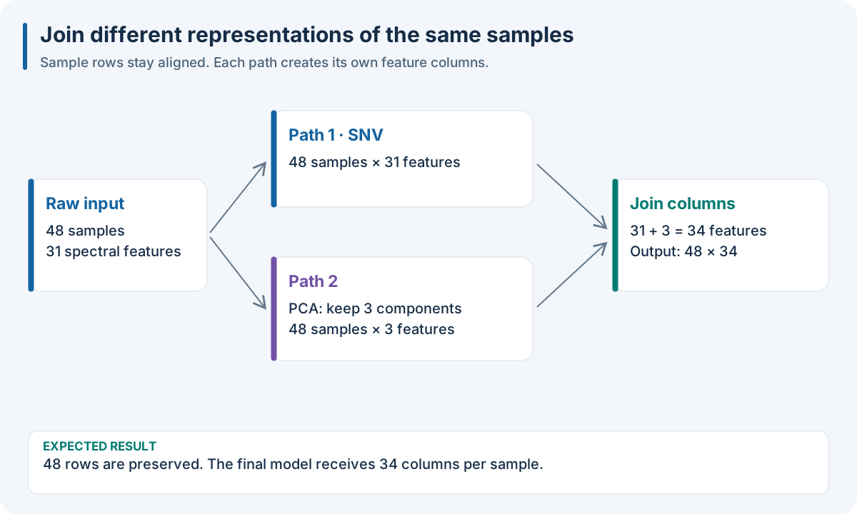
Observation count stays fixed. Output width is the sum of block widths: 31 + 3 = 34.
Note
These tabs express the same Python SDK workflow. JSON and YAML are recipe files; Python can also use sklearn/nirs4all objects. R, Octave and WASM native pipeline facades do not execute this host-controller node directly. For a recipe that runs in those languages, use 10. Run the same recipe in your language.
{
  "pipeline": [
    {
      "split": {
        "class": "sklearn.model_selection.KFold",
        "params": {
          "n_splits": 3,
          "shuffle": true,
          "random_state": 17
        }
      }
    },
    {
      "concat_transform": [
        {
          "class": "nirs4all.operators.transforms.StandardNormalVariate"
        },
        {
          "class": "sklearn.decomposition.PCA",
          "params": {
            "n_components": 3
          }
        }
      ]
    },
    {
      "model": {
        "class": "sklearn.linear_model.Ridge",
        "params": {
          "alpha": 1.0
        }
      }
    }
  ]
}
pipeline:
- split:
    class: sklearn.model_selection.KFold
    params:
      n_splits: 3
      shuffle: true
      random_state: 17
- concat_transform:
  - class: nirs4all.operators.transforms.StandardNormalVariate
  - class: sklearn.decomposition.PCA
    params:
      n_components: 3
- model:
    class: sklearn.linear_model.Ridge
    params:
      alpha: 1.0
import tempfile
import numpy as np
import nirs4all
from nirs4all.data.dataset import SpectroDataset
from sklearn.model_selection import KFold
from sklearn.decomposition import PCA
from sklearn.linear_model import Ridge
from nirs4all.operators.transforms import SNV

rng = np.random.default_rng(17)
X = rng.normal(size=(48, 31))
y = 2 * X[:, 10] - X[:, 20] + rng.normal(scale=0.1, size=48)
dataset = SpectroDataset("worked_node")
dataset.add_samples(X[:40], {"partition": "train"},
                    headers=[str(i) for i in range(31)])
dataset.add_samples(X[40:], {"partition": "test"})
dataset.add_targets(y.reshape(-1, 1))


pipeline = [
    KFold(n_splits=3, shuffle=True, random_state=17),
    {"concat_transform": [SNV(), PCA(n_components=3)]},
    {"model": Ridge(alpha=1.0)},
]
with tempfile.TemporaryDirectory() as workspace:
    result = nirs4all.run(pipeline, dataset, engine="legacy",
                         workspace_path=workspace, save_charts=False, verbose=0)
    print("CV validation score:", result.cv_best_score)
    print("Selected model test RMSE:", result.best_rmse)
    result.close()
What to expect: 31 SNV features plus three PCA scores make 34 columns for
Ridge. All 48 observation identities and targets remain. PCA learns its axes
from training data; new rows use saved axes.
The standalone example explicitly selects engine="legacy", where this
controller is available. Use independently held-out evaluation when comparing
learned feature constructions.
What each list level means
Entry inside |
Meaning |
|---|---|
Transformer |
One parallel block |
Nested list |
Sequential chain forming one parallel block |
Nested |
Parallel concatenation inside a block |
|
Pass through incoming features |
Keep 31 raw wavelengths and add three PCA scores after SNV:
{
  "pipeline": [
    {
      "split": {
        "class": "sklearn.model_selection.KFold",
        "params": {
          "n_splits": 3,
          "shuffle": true,
          "random_state": 17
        }
      }
    },
    {
      "concat_transform": [
        null,
        [
          {
            "class": "nirs4all.operators.transforms.StandardNormalVariate"
          },
          {
            "class": "sklearn.decomposition.PCA",
            "params": {
              "n_components": 3
            }
          }
        ]
      ]
    },
    {
      "model": {
        "class": "sklearn.linear_model.Ridge",
        "params": {
          "alpha": 1.0
        }
      }
    }
  ]
}
pipeline:
- split:
    class: sklearn.model_selection.KFold
    params:
      n_splits: 3
      shuffle: true
      random_state: 17
- concat_transform:
  - null
  - - class: nirs4all.operators.transforms.StandardNormalVariate
    - class: sklearn.decomposition.PCA
      params:
        n_components: 3
- model:
    class: sklearn.linear_model.Ridge
    params:
      alpha: 1.0
from nirs4all.operators.transforms import StandardNormalVariate as SNV
from sklearn.decomposition import PCA
from sklearn.linear_model import Ridge
from sklearn.model_selection import KFold

pipeline = [{'split': KFold(n_splits=3, shuffle=True, random_state=17)},
 {'concat_transform': [None, [SNV(), PCA(n_components=3)]]},
 {'model': Ridge(alpha=1.0)}]
Expected result: 34 columns, but the last three now summarize SNV-normalized spectra. The first example’s PCA scores summarize raw spectra. Same shape, different scientific meaning.
Options and checks
The short list form is usually sufficient. The detailed mapping supports
operations, output name and source_processing to select an input view.
Sum output widths before fitting: twenty 31-column blocks make 620 features, not twenty observations.
More columns can give a block more influence. Check units, scaling and redundancy.
Every block must preserve the same row IDs and row order.
Different-width blocks are allowed when concatenated; different row counts are not.
Runnable context: U02 feature augmentation. Full option schema: Pipeline Keywords Reference.